User:Sunitinagpurkar/My sandbox

Theories of Profit

Theories of Profit

Introduction

	Learning Objectives
After reading this chapter, you are expected to learn about:

Definition

Assumptions

1. There are two factor inputs labour and capital
2. The proportions of factor are variable.
3. Physical production conditions are given
4. The Scale of operation is variable
5. The state of technology remains constant

The shape of Isoquant

In this section we examine the characteristics of isoquants, define the economic region of production and consider the special cases where the commodities can only be produced with least cost factor combination.

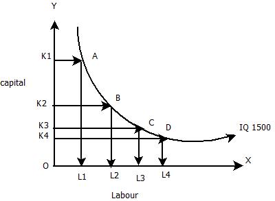
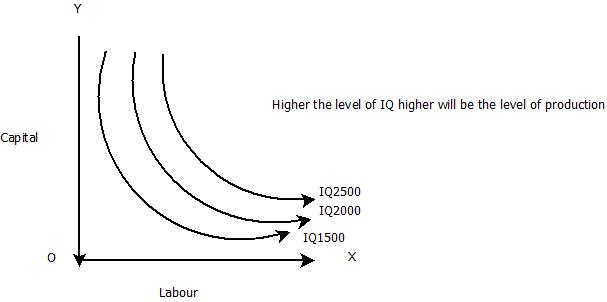
We can see that the shape of isoquant plays an important a role in the production theory as the shape of indifference curve in the consumption theory. Iso quant map shows all the possible combinations of labour and capital that can produce different levels of output. The iso quant closer to the origin indicates a lower level of output. The slope of iso quant is indicated as [math]\frac{K}{L}[/math]=MRSLk=[math]\frac{MPL}{MPk}[/math]

Table indicating various combinations of Labour and Capital to produce 1500 Units of Output

COMBINATIONS	UNITS OF CAPITAL	UNITS OF LABOUR	TOTAL OUTPUT
A	50(OK)	1 (OL1)	1500(IQ1)
B	45(OK2)	2(OL2)	1500(IQ1)
C	41(OK3)	3(OL3)	1500(IQ1)
D	38(OK4)	4(OL4)	1500(IQ1)

Properties/Characteristics of Isoquants

Isoquants, abbreviated as IQs, possess the same properties as those of the indifference curves. For the convenience of the students, we can state them as follows.

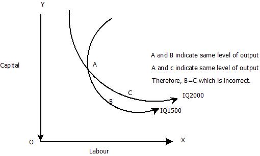
1. Two isoquants do not intersect each other:

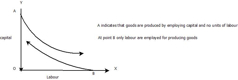
1. No isoquant can touch either axis

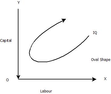
1. Isoquant is oval in shape

1. A higher IQ implies a higher level of output

1. IQs are never parallel to each other. Interspacing between them is least at the ends and maximum in the middle.
2. IQs are convex to the origin: convex isoquants possess continuous substitutability of K and L over a stretch. Beyond this stretch, K and L are not substitutable foe each other.
3. IQs may be linear when labour and capital are perfect substitute. A linear isoquant implies that either factor can be used in proportion. If isoquant has several linear segments separated by kinks, the isoquant is called kinked isoquant or activity analysis isoquant or linear programming isoquant. Such isoquants are used in linear programming.
4. If Land K are prefect complements to each other, the IQ is L-shaped. Such isoquant is known a input-output isoquant or Leontief isoquant. There is only one combination of L and K available for production. It is the corner point of L-shaped isoquant.
5. If marginal product of one of the two factors is zero, IQ is parallel to the axis on which the factor with zero marginal products is represented.
6. If one of the two factors has negative marginal product the IQ slopes upwards from left to right.
7. If both the factors have negative marginal products, the IQ is concave to the origin.
8. If the producer has a preference for a factor of production, the IQ is quasi linear.
9. If the factors to be employed in whole numbers units only. The IQ is discontinuous.

Isocost curves:

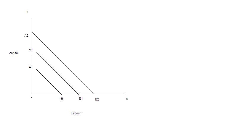
Isocost curve is the locus traced out by various combinations of L and K, each of which costs the producer the same amount of money (C ) Differentiating equation with respect to L, we have dK/dL = -w/r This gives the slope of the producer’s budget line (isocost curve). Iso cost line shows various combinations of labour and capital that the firm can buy for a given factor prices. The slope of iso cost line = PL/Pk. In this equation , PL is the price of labour and Pk is the price of capital. The slope of iso cost line indicates the ratio of the factor prices. A set of isocost lines can be drawn for different levels of factor prices, or different sums of money. The iso cost line will shift to the right when money spent on factors increases or firm could buy more as the factor prices are given.

Slope of iso cost line

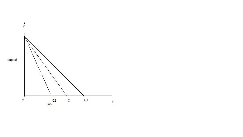
With the change in the factor prices the slope of iso cost lien will change. If the price of labour falls the firm could buy more of labour and the line will shift away from the origin. The slope depends on the prices of factors of production and the amount of money which the firm spends on the factors. When the amount of money spent by the firm changes, the isocost line may shift but its slope remains the same. A change in factor price makes changes in the slope of isocost lines as shown in the figure.

Least Cost Factor Combination or Producer’s Equilibrium or Optimal Combination of Inputs

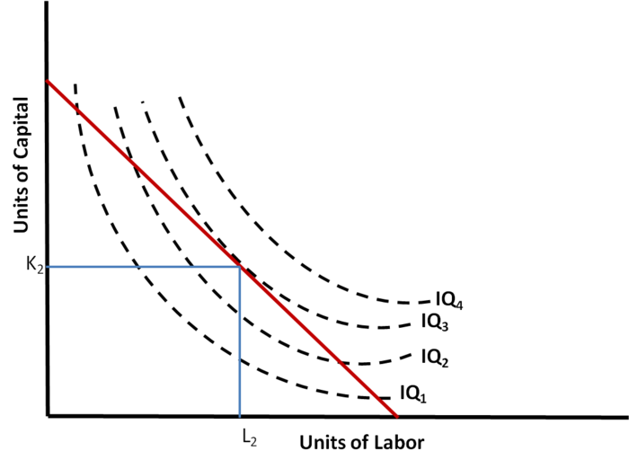
The firm can achieve maximum profits by choosing that combination of factors which will cost it the least. The choice is based on the prices of factors of production at a particular time. The firm can maximize its profits either by maximizing the level of output for a given cost or by minimizing the cost of producing a given output. In both cases the factors will have to be employed in optimal combination at which the cost of production will be minimum. The least cost factor combination can be determined by imposing the isoquant map on isocost line. The point of tangency between the isocost and an isoquant is an important but not a necessary condition for producer’s equilibrium. The essential condition is that the slope of the isocost line must equal the slope of the isoquant. Thus at a point of equilibrium marginal physical productivities of the two factors must be equal the ratio of their prices. The marginal physical product per rupee of one factor must be equal to tht of the other factor. And isoquant must be convex to the origin. The marginal rate of technical substitution of labour for capital must be diminishing at the point of equilibrium.

The Economic region of production

The firm would not operate on the positively sloped portion of an isoquant because it could produce the same level of quantity with less capital and labour. Economic region of Production:

Ridge lines: separate the relevant (i.e. negatively sloped) from the irrelevant (or the positively sloped) portion of the isoquant.

Ridge lines joins points on the various isoquants where the isoquants have zero slope (and thus zero MRTSlk) .

Case Study

Enter your text here

	Activity
Write your activity here

Example: {{{Example}}}

	Self-Assessment Questions (SAQs) {{{n}}}
{{{SAQ}}}

Multichoice Questions

1. Iso quants are equal revenue lines (a) True (b) False 2. Iso quant is sloping downwardso when inputs are used in fixed proportion (a) True (b) False 3. Iso quant is also known as Production indifference curve (a) True (b) False 4. A higher isoquant represent lower level of output. (a) True (b) False 5. Least cost input is a combination where the slope of isoquant is equal to the slope of isocost (a) True (b) False Your score is 0 / 0

Results

An isoquant shows the various combination of two inputs that can be used to produce a specific level of output. From the isoquant map, we can generate the total product curve of each input by holding the quantity of the other input constant.

Isoquants are negatively sloped in the economically relevant range, convex to the origin and do not intersect. The absolute value of the slope of Isoquant is called the Marginal Rate of Technical Substitution. This equals the ratio of marginal productivity of two inputs.

As we move down along an isoquant the absolute value of its slope or Marginal Rate of Technical Substitution declines and the isoquant is convex. Ridge lines separate the relevant (i.e. the negatively sloped) from the irrelevant (or positively sloped) portion of the isoquant. 

With right angled or L shaped, isoquant , inputs can only be combined in fixed proportion in production.

Key Terms

Iso Quant

Iso cost

Ridge Lines

Least Cost Combination

Producers Equilibrium

Marginal Rate of Technical Substitution

Extension exercise

Enter your text here

21, November 2024

}-

Last name	First Name	Gender	Institution	Designation	Username
Singh	Dr. Savithri	Female	Acharya Narendra Dev College	Principal	User:Savi.odl	Facilitator
Toteja	Dr. Ravi	Male	Acharya Narendra Dev College	Associate Professor - Zoology	User:Rtoteja27	Facilitator
Misra	Dr. Neeti	Female	Acharya Narendra Dev College	Associate Professor - Chemistry	User:Neeti m	Facilitator
Dhopte	Dr Sujata	Female	Malini Kishor Sanghvi College of Commerce & Economics	Assistant Professor - Economics	User:Dr Sujata Dhopte	Participant
Mishra	Sanghamitra	Female	SIWS College	Assistant Professor	user:Sanghamitra	Participant
Aggie	Dr. Menezes	Male	St. Xavier's College, Mumbai	Associate Professor	user:aggie menezes	participant
V	Jayasree.	Female	Sree Narayana Guru College	Associate Professor-  Economics	user:jayasreev	Participant
Keshav	GHORUDE	Male	A. V. College of Arts	Associate Professor	User:Kngvartak	Participant
Shukla	Dr. Smita	Female	University of Mumbai	Associate Professor - Management	User:smitashukla	Participant
Mahadeshwar	Rekha	Female	S.I.W.S. N.R. Swamy College	Associate Professor	user:Rekham	Participant
Nandola	Rajan J.	Male	Thakur College of Science and College	Assistant Professor - Economics	User:Rajan Nandola	Participant
Ganapathy	Saroja	Female	Ramnarain Ruia College	Assistant Professor of English	User:Saga30	Participant
Rajalakshmy	Dr G	Female	L S Raheja College	Associate Professor Economics	User:Rajalakshmy	Participant
Kasibhotla	Venkateswarlu	Male	Associate Professor, Economics	L S Raheja College	User:Kvenkatesh	Participant
Bhagwat	Dr. Hemangi	Female	NSS College of Commerce	Principal	User:Hemangi	Participant
SAWANT	SURESH	Male	L S RAHEJA COLLEGE	ASSOCIATE PROF	User:SMSAWANT	Participant
Nakhare	Kirti	Female	SIWS College	Assistant Professor of English	User:kirtiynakhare	Participant
Malwade	Varsha	Female	Ramnarain Ruia College	Associate Professor, Economics	User:Varsha Malwade	Participant
Phadnis	Dr.Sadhana	Female	ICLES M J College	Associate Professor	User:Sadhana	Participant
Narayanaswamy	Meenakshi	Female	G.N.Khalsa college	Associate professor,Economics	user:Meenakshi narayanaswamy	Participant
Gala	Asha	Female	S.I.E.S college	Associate professor,Economics	user:asha gala	Participant
Gadgil	Gayatri	Female	DG Ruparel College	Assistant Professor- English	User:CommSkills	Participant
Deshmukh	Mahadeo	Male	S K Somaiya College of ASC	Assistant Professor	User:Deshmukhms	Participant
Vibhute	Somnath	Male	St. Gonsalo Garcia College Vasai	Assistant Professor	User:somnath11	participants
Mathur	Rajani	Female	S I E S College of Arts Science and Commerce	Associate Professor	User:Rajani	Participants
Laghate	Kavita	Female	Jamnalal Bajaj Institute of Management Studies University of Mumbai	Associate Professor	user:kavita11	co-ordinator

References and Bibliography

1. Principles of Microeconomics,Dominick Salvatore Fifth Edition, Oxford International Student Edition.
2. Micro Economics:Edwin Mansfield and Gary Yohe,Tenth Edition, Published by W.W. Norton & Company
3. Economics:Samuelson and Nordhaus,Eighteenth Edition, Published by Tata McGraw Hill

Further Readings