User:Chela5808/My sandbox Sam4 HandStyled
| Before Styling | Sample 1 | Sample 2 | Sample 3 | Sample 4 | Sample 5 | Sample 6 |
| After Styling | Sample 1 | Sample 2 | Sample 3 | Sample 4 | Sample 5 | Sample 6 |
Styling by hand Sample 4
- Text: Wiki Markup;
- Formulae: [math]\mathrm{L\!\!^{{}_{\scriptstyle A}} \!\!\!\!\!\;\; T\!_{\displaystyle E} \! X} \,[/math] some took directly from corresponding .tex file.
Comments:
- Hand styling time : 1.5 hrs
Example
As an example of how things go, you can look at the function
and find the two first derivatives, one for each of the two variables. Thus
[math]\left (\frac{\partial f}{\partial x}\right)_y =2x-2y,\qquad \left (\frac{\partial f}{\partial y}\right)_x =-2x-6y\,[/math]
It’s easy; all you have to do is differentiate with respect to one variable, treating the other just as if it were a constant. And with only two independent variables you can even drop the subscripts, which only mean “the other one”. That’s what we’ll do from now on.
Now try some of the Exercises at the end of the Chapter.
Towards the end of Section 2.3, in talking about functions of only one variable, we were able to define ‘higher’ derivatives by differentiating the ‘first’ derivative to get ‘second’ and ‘third’ derivatives: [math]\text{d}^2f/\text{d}x^2\,[/math] and [math]\text{d}^3f/\text{d}x^3\,[/math], etc.; and we can do the same for functions of more than one variable. Thus, if [math]z=f(x,y)\,[/math] we can find first derivatives, such as [math](\partial f/\partial x)\,[/math] in (??), and then go on to get
| [math]\left (\frac{\partial^2 f}{\partial x^2}\right)=\left (\frac{\partial }{\partial x}\right)\left (\frac{\partial f}{\partial x}\right),\qquad \left (\frac{\partial^2 f}{\partial x \partial y}\right)=\left (\frac{\partial }{\partial x}\right)\left (\frac{\partial f}{\partial y}\right),\,[/math] | (6) |
and so on.
We have to take care with the order of the differentiations: usually, in
the operation nearest the function [math]f\,[/math] is the one you do first – but some books use the opposite rule, so watch out!. The rule used here is close to the one in which the operators [math]\mathsf{D}_x,\mathsf{D}_y[/math] are used. The second derivative we’re talking about can be written in this way as [math]\mathsf{D}_x\mathsf{D}_y f\,[/math] , which is simpler and clearer. And, just as with functions of one variable, we can make things even easier: the notations for first derivatives are
| [math]\left (\frac{\partial f}{\partial x}\right)=\mathsf{D}_x f=f_x\,,\qquad \left (\frac{\partial f}{\partial y}\right)=\mathsf{D}_y f=f_y \,,\,[/math] | (7) |
while for the second derivatives we have
| [math]\left (\frac{\partial^2 f}{\partial x^2}\right)=\left (\frac{\partial }{\partial x}\right)\left (\frac{\partial f}{\partial x}\right)=\mathsf{D}_x \mathsf{D}_xf=f_{xx}\,[/math] | (8) |
and
| [math]\left (\frac{\partial^2 f}{\partial x\partial y}\right)=\mathsf{D}_x \mathsf{D}_yf=f_{xy}\,[/math] | (9) |
(Notice that we don’t need to put primes on the derivatives, one each time we differentiate, because the subscripts on [math]f_x\,,f_{xy}\,,\,[/math] in (??) and (??), tell us which differentiations we’ve done and how many.) The older books use the full notation, on the left in these equations, which goes back to Leibnitz and the early days of the Calculus, but we’ll often use the simpler forms shown on the right. So be sure you know about them all.
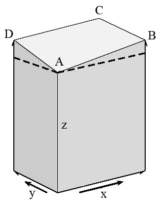
You can see what the derivatives mean, with the help of Fig.24, which shows what happens when [math]x\rightarrow x+\text{d}x\,[/math] and [math]y\rightarrow y+\text{d}y\,[/math].
Example. Let’s find some second derivatives for a function of the third degree.
[math]z=f(x,y)=x^3+4x^2y-6xy^2-2 y^3.\,[/math]
Differentiating, we get first derivatives
[math](\partial f/\partial x)= 3x^2+8xy -6y^2,\;(\partial f/\partial y)= 4x^2 -12xy - 6y^2,\,[/math]
and differentiating again we find four second derivatives:
| [math]\left(\frac{\partial^2 f}{\partial x^2}\right) = 6x + 8y, [/math] | [math]\left(\frac{\partial^2 f}{\partial x \partial y}\right) = 8x -12y,[/math] |
| [math]\left(\frac{\partial^2 f}{\partial y \partial x}\right) = 8x -12y,[/math] | [math]\left(\frac{\partial^2 f}{\partial y^2}\right) = -12x -12y.[/math] |
Note that in the ‘mixed’ derivatives, where you differentiated once with respect to [math]x\,[/math] and once with respect to y, the results came out to be exactly the same: it didn’t matter which one you did first. This is true for all the functions we have called “well behaved” (meaning there is a unique value of the dependent variable [math]z\,[/math] for every choice of the independent variables, the function is continuous and smooth, and so on).
Figure 24 shows four neighbouring points [math]\text{A, B, C, D}\,[/math] on the surface: they are vertically above the corners of the rectangle at the bottom of the picture, which lies in the horizontal xy-plane. The broken lines indicate a plane passing through [math]\text{A}\,[/math], parallel to the base, so you can see the slopes of the edges of the sloping face. Thus, the slopes of [math]\text{AB}\,[/math] and [math]\text{AD}\,[/math] are
[math]\mathrm{slope}_{\mathrm{AB}}= \left(\frac{\partial f}{\partial x}\right) =\mathsf{D}_x\,f = f_x(x,y),[/math]
[math]\mathrm{slope}_{\mathrm{AD}}= \left(\frac{\partial f}{\partial y}\right) =\mathsf{D}_y\,f = f_y(x,y).[/math]
Here the forms on the right show also the variables for Point [math]\text{A}\,[/math] where the derivatives are evaluated. The slope of side [math]\text{BC}\,[/math], at Point [math]\text{B}\,[/math] will be
[math]\mathrm{slope}_{\mathrm{BC}} = \left(\frac{\partial f}{\partial y}\right) =\mathsf{D}_y\,f = f_y(x+\text{d} x,y). [/math]
Notice that this is the slope in the [math]\text{y}\,[/math] direction, where only [math]\text{x}\,[/math] is changing, but it is evaluated using the variables for Point [math]\text{B}\,[/math]. Why do
