Working with spreadsheets/Spreadsheet calculations/Functions

Working with Spreadsheets

Basic skills applicable to planning, creating and formatting an Excel spreadsheet.
An OP Online course from the National Certificate in Computing (Level 2) programme.

About this course  |  Getting started  |  Course schedule  |  Assessment overview  |  Help

A function is a pre-defined formula that’s already in Excel. If you have a choice, use a function over a formula.

Activity

Please note: the following link will open in a new window/tab. When you have finished, simply close the window/tab and you'll return to this page. Work through the tutorial on Working with Basic Functions Don't forget to check out the video on page 2.

Activity

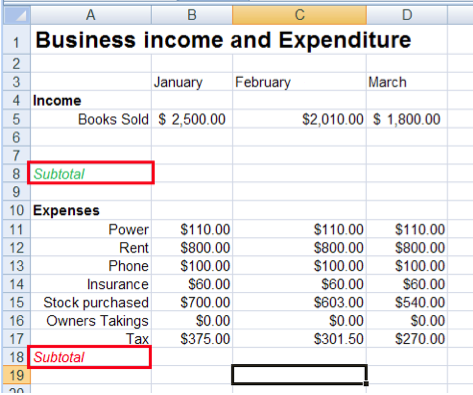
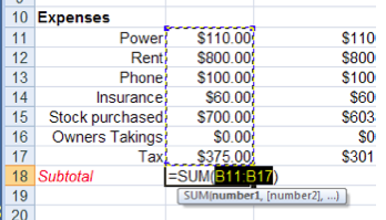
Open your bookshop spreadsheet. We are going to add some formulae, add some functions and use the spreadsheet to provide new information. Add two new headings in cells A8 and A18 called Subtotal. Use the Font group to apply italic formatting. We’re also going to use the font colour button. Choose green for the income subtotal and red for the expenses subtotal. We are now going to add a function to add up all our expenses. Click in Cell B18. Use Home Tab > Editing Group and locate the Autosum button. From the drop-down menu choose Sum. Excel will automatically insert the SUM function into cell B18. It should also correctly choose the range B11:B17. Press ENTER on your keyboard. We also want to have a subtotal under the columns for February and March. Use what you know of coying and pasting to copy the forumula to the correct place in the next two columns. Apply italics, currency formatting and colour these subtotals red. 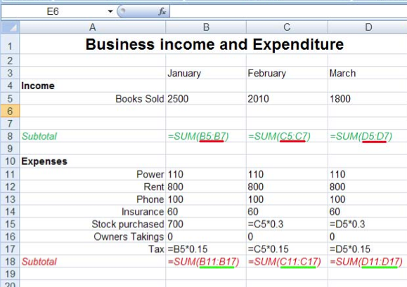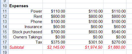If you click in each cell that contains a subtotal, you should notice that the cell ranges that have been selected also change. Here is a picture to show you: We can see that copying and pasting a formula automatically amends the cell ranges - very handy! Now click in cell B8. We are going to add a SUM function here as well. 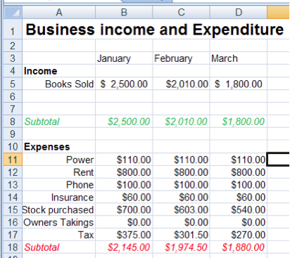Copy the sum function across the next 3 columns. Format these subtotals to be italic, currency and green. Your finished subtotals should look like: Save your work. We can see by looking that on the whole, we should have a positive balance at the end of each month, but how much? 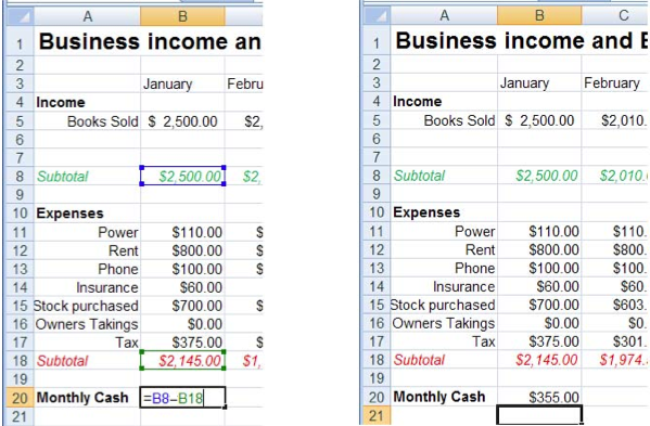If we look at January and grab a calculator, we should have: 2500.00 – 2145.00 = $355 Let’s make Excel do the donkey-work: In cell A20 type Monthly Cash. Left-align this heading. If we look at our workings-out from above, we can see that we’ve used the value stored in B8 and subtracted the value stored in B18. We can see the beginnings of a formula that we can use. In cell B20 type in =B8-B18. Press Enter. We should have the answer of $355 appear. Copy your formula across to provide monthly cash totals for February and March. Save your work and close Excel.

Other functions

Here is a brief explanation of the other functions that you can access from the Autosum (Σ) button:

=sum(A1:A6)

Adds up or sums the numbers in the range provided

=average(A1:A6)

Works out the average of the cell values in the range

=Max(A1:A6)

Returns the maximum value stored in the range

=Min(A1:A6)

Returns the minimum value stored in the range

=Count(A1:A6)

Counts the number of cells that contains numbers only in the range

=Counta(A1:A6)

Counts the number of cells that are not empty (different to the one above)

Summary

So far in this unit, you have learned how to:

• Add new data to your spreadsheet
• Apply formats like currency, colour, italics
• Create formulae to perform basic maths
• Use Excel functions
• Copy and pasted formulae and functions
• Provided a solution to a simple problem

|