Equations of State
| Thermodynamics | |
|---|---|
| Introduction | What is this thing called Thermodynamics??? | Definitions | Thermal Equilibrium and Zeroth Law | Limitations |
| First Law | Work, Heat, Energy, and the First Law | Work, Heat, Energy, and the First Law (simplied) | Derivatives | Derivatives Exercise | Reversibility, Enthalpy, and Heat Capacity |
| Second Law | Things to Think About | Observations and Second Law of Thermodynamics | Alternative Approach - the Clausis Inequality | Consequences of the Second Law | Consequences of the Second Law (simplified) | Carnot Principle - motivation and examples | Equivalence of Second Law Statements* |
| Third Law | Third Law of Thermodynamics | Consequences of Third Law* |
| Development of Thermodynamics | The Thermodynamic Network | Network Exercise | Equations of State (EOS) | EOS Example, Reading Tables, and Numerical Analysis | EOS Exercises | Thermochemistry |
* Optional Section | |
| Learn how to develop the relationship between pressure, volume, and temperature through the use of eqations of state |
Contents
Introduction and Motivation
In the last two sections we looked at the thermodynamics network. We said that we needed two things to determine relations between properties:
- Pressure-Volume-Temperature (PVT) Data
- Heat Capacity Data
This section will look at PVT data. We will look at heat capacity data later.
| Equation of State The relationship between pressure, volume, and temperature for a given substance |
There are three ways of expressing PVT data:
- Experimental Data (usually given in tables)
- Generalized Correlations
- Analytical Equations
Definitions
Compressibility Factor
The Compressibility Factor, Z is given by,
[math]Z=\frac{P\hat{V}}{RT}[/math]
where R = gas constant = 8.314 J/mol K = 83.14 cm3 bar/mol K
Two important notes about compressibility factors:
- Z is dimensionless
- Z is not a constant. Students often forget this.
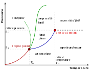
Critical Point
The Critical Point is the point above which there exists no phase boundaries. A gas above the critical point will not form a liquid if it is isothermally compressed.
Critical Constants
The Critical Constants are the values of properties at the critical points (for example, critical temperature).
We use a subscript C to denote a critical constant. For example, TC, PC.
Reduced Properties
Reduced Properties are the value of a property divided by its corresponding critical constant. We use a subscript of R to denote a reduced property.
For example,
[math]T_R = \frac{T}{T_C}[/math]
[math]P_R = \frac{P}{P_C}[/math]
Phase Rule
To understand what parameters are important in PVT relations, we need to understand the concepts of degrees of freedom and the phase rule. They are also important for phase equilibrium.
| Degrees of Freedom The number of independent, intensive variables required to determine the state of a system |
Phase Rule
[math]F=C+2-P[/math]
where F = degrees of freedom, C = number of components, P = number of phases}}
Example
Let us first consider water at room temperature. We have one component (water) and only one phase (liquid), therefore the degrees of freedom is
F = 1 + 2 - 1 = 2
We have two degrees of freedom, therefore we can independently set two variables -- say pressure and temperature. So we can have water at 1 bar, 25 °C; 1 bar, 80 °C; or 5 bar, 25 °C.
Now let us consider boiling water. We still have one component, but we now have two phases (liquid and vapor). The number of degrees of freedom is now:
F = 1 + 2 - 2 = 1
We have only one degree of freedom, therefore we can set only one independent variable -- pressure or temperature. We all know that at one atmosphere, the boiling point is 100 °C, not 80° or 120 °.
Real Gases
The figure on the right shows how a real gas behaves with respect to pressure, temperature, and volume.
The dome-shaped region is where there are two phases -- liquid and vapor[1]. To the left there is only liquid present, whereas to the right there is only vapor present. The top of the dome is the critical point. [2]
The lines that go roughly left-to-right are isotherms -- lines of constant temperature. Note that the isotherms are horizontal inside the two phase region. Remember the phase rule? Here F = 1, therefore the pressure and temperature are not independent.
At the critical point the following two relations apply:
[math]\left(\frac{\partial P}{\partial V}\right)_{T_{C}}=0[/math] [math]\left(\frac{\partial^{2}P}{\partial V^{2}}\right)_{T_{C}}=0[/math]
Generalized Correlations
Theory of Corresponding States
The compressibility factor does not correspond well with absolute temperature or pressure. However, we can correlate Z to reduced temperature and pressure:
[math]Z=f\left(T_{R},P_{R}\right)[/math]
This is called the theory of corresponding states.
A Third Parameter
Only a few fluids show behavior that agrees with the theory of corresponding states. These are called simple fluids.
Most fluids (normal fluids) show some deviation from simple fluids. This suggests a third parameter needs to be added to account for this deviation.
Kenneth Pitzer introduced a third parameter based on vapor pressure. He called it the acentric factor, ω:
[math]\omega=-1.0-\log_{10}\left(P_{R}^{sat}\right)_{T_{R}=0.7}[/math]
where [math]\left(P_{R}^{sat}\right)_{T_{R}=0.7}[/math] is the reduced vapor pressure at TR = 0.7
Notice that ω is chosen such that it equals zero for simple fluids.
The Pitzer acentric factor is used with the theory of corresponding states as:
[math]Z=Z^{0}\left(P_{R},T_{R}\right)+\omega Z^{1}\left(P_{R},T_{R}\right)[/math]
where Z0 is Z for simple fluids and Z1 is the deviation.
In the next section we will see how to apply this equation.
Analytical Equations
The theory of corresponding states is very good, except for highly polar substances (including water). However, there are times where we would prefer to use analytical equations of state. The most important of these is where we wish to do computer calculations.
van der Waals Equation
J. D. van der Waals[3], in 1873, developed the first analytical equation of state. He started with the ideal gas equation, [math]P\hat{V} = RT[/math], and then added two corrections based on theory:
- The ideal gas equation assumes that molecules do not interact. Of course, molecules interact by the van der Waals force. This interaction reduces the pressure since the attraction between molecules reduces the chance of them hitting the wall of the container.
- The ideal gas assumes that molecules have no volume. But particles do have a physical size. This physical presence therefore reduce the volume through which the particles move.
If we apply these two corrections we get the van der Waals equation:
[math]P=\frac{RT}{\hat{V}-b}-\frac{a}{\hat{V}^{2}}[/math]
To determine a and b, van der Waals used the properties at the critical point [math]\left(\frac{\partial P}{\partial V}\right)_{T_{C}}=0 \text{ and } \left(\frac{\partial^{2}P}{\partial V^{2}}\right)_{T_{C}}=0[/math] to give:
[math]a=\frac{27R^{2}T_{C}^{2}}{64P_{C}} \qquad b=\frac{RT_{C}}{8P_{C}}[/math]
Cubic Equations
van der Waals equation is called a cubic equation – that is it is cubic in volume.
Other, more accurate, cubic equations are commonly used. These are all based on the van der Waals equation. Let us now go through some of these equations.
Redlich-Kwong Equation
Redlich and Kwong improved the van der Waals equation by making a dependent on temperatures.
[math]P =\frac{RT}{\hat{V}-b}-\frac{a}{T^{0.5}\hat{V}(\hat{V}-b)}[/math]
[math]a =\frac{0.42748R^{2}T_{c}^{2.5}}{P_{C}} \qquad b =\frac{0.08664RT_{C}}{P_{C}}[/math]
Soave and Peng-Robinson Equations
Soave, and Peng and Robinson improved further the van der Waals equation by using the Pitzer acentric factor and fitting a to hydrocarbon data.
The Soave equation is
[math]P =\frac{RT}{\hat{V}-b}-\frac{a}{\hat{V}(\hat{V}+b)}[/math]
[math]a =\frac{0.42748R^{2}T_{c}^{2}}{P_{C}}\left[1+f\left(1-T_{R}^{0.5}\right)\right]^{2} \qquad b=\frac{0.08664RT_{C}}{P_{C}} \qquad f=0.48+1.574\omega-0.176\omega^{2}[/math]
The Peng-Robinson equation is
[math]P =\frac{RT}{\hat{V}-b}-\frac{a}{\hat{V}^{2}+2b\hat{V}-b^{2}}[/math]
[math]a =\frac{0.45724R^{2}T_{c}^{2}}{P_{C}}\left[1+f\left(1-T_{R}^{0.5}\right)\right]^{2} \qquad b=\frac{0.08664RT_{C}}{P_{C}} \qquad f =0.37464+1.54226\omega-0.26992\omega^{2}[/math]
Other Equations
Viral Equation
Statistical mechanics suggests that we can write the compressibility factor as a power series in 1/V:
[math]Z=1+\frac{B}{\hat{V}}+\frac{C}{\hat{V}^{2}}+\frac{D}{\hat{V}^{3}}+\ldots[/math]
As the above would require infinite number of parameters, it is usually truncated to two or three terms:
[math]Z = 1+\frac{B}{\hat{V}}+\frac{C}{\hat{V}^{2}} \text{ or } Z = 1+\frac{B}{\hat{V}}[/math]
The coefficients B and C are known as the second and third viral coefficients, respectively. They are usually give in tables.
For nonpolar fluids the following correlation can be used:
[math]\frac{BP_{C}}{RT_{C}}=B^{0}+\omega B^{1} \qquad B^{0}=0.083-\frac{0.422}{T_{R}^{1.6}} \qquad B^{1}=0.139-\frac{0.172}{T_{C}^{4.2}}[/math]
Benedict-Webb-Rubin Equation
The Benedict-Webb-Rubin (BWR) equation is based on the viral equation but with an additional exponential term. This is more accurate than the above, but also more complex.
[math]P=\frac{RT}{\hat{V}}+\frac{B_{0}RT-A_{0}-C_{0}/T^{2}}{\hat{V}^{2}}+\frac{bRT}{\hat{V}^{3}}+\frac{a\alpha}{\hat{V}^{6}}+\frac{c}{\hat{V}^{3}T^{2}}\left(1+\frac{\gamma}{\hat{V}^{2}}\right)\exp\left(\frac{-\gamma}{\hat{V}^{2}}\right)[/math]
where A0, B0, C0, a, b, c, α, γ are constants which depend on the type of substance
Recommendations
If possible use the three parameter correlation (i.e. theory of corresponding states with the Pitzer acentric factor) and the Z tables. They are the most accurate.
For most applications the van der Waals equation is sufficiently good.
The Soave or Peng-Robinson equation are the most commonly used equations in engineering. Use these for higher pressures or if you have access to a computer program.
The viral equation can only be used for gases at low pressure where V > 2VC. The equation is not accurate at higher pressures.
The Redlich-Kwong equation is no longer used.
The BWR equation is very good, but constants are only available for a few chemicals.
None of these equations are accurate near the critical point.

