User:Rekham/My Sandbox
MICROECONOMICS

|
PRICE EFFECT |

|
Introduction |
At the market place a consumer faces market conditions that change constantly. Some times there is increase in the price of a good or there is decrease in the price. As a policy change new taxes are imposed on goods or the goods are subsidized. These situations lead the consumer to change her/his consumption, in order to maximize the utility of spendable income.
In term of indifference curves analysis,as explained in the section on CONSUMER'S EQUILIBRIUM, we have seen how the optimal consumption combination, the one that maximizes the utility of consumer's spendable income, is determined at the point where budget constraint is tangent to an indifference curve. The price effect on the other hand measures consumer movement from one optimal consumption combination to another, on her/his indifference map, as a result of change in the price of a good.
| Price Effect |
The price effect represents change in consumer’s optimal consumption combination on account of change in the price of a good and thereby changes in quantity purchased, price of another good and consumer’s income remaining unchanged. The consumer is better-off when optimal consumption combination is located on a higher indifference curve and vice versa. In the words of Lipsey," The price effect shows how much satisfaction of the consumer varies due to the change in the consumption of two goods, as the price of one changes, the price of the other and money income remains constant." []
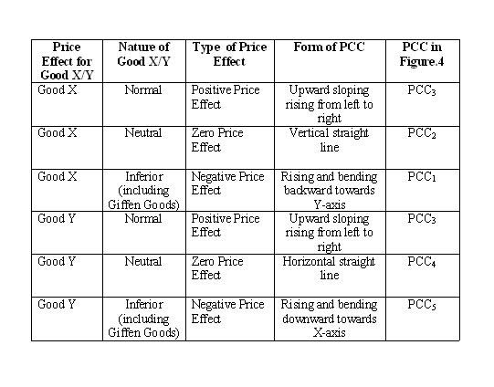
Understand that a consumer's responses to a price change differ depending upon the nature of a good, viz. a normal good, inferior good or a neutral good. Accordingly we have different types of price effects such as positive, negative and zero price effects. These types of price effect corresponding to consumer's responses for different nature of goods are summarized in chart.1:
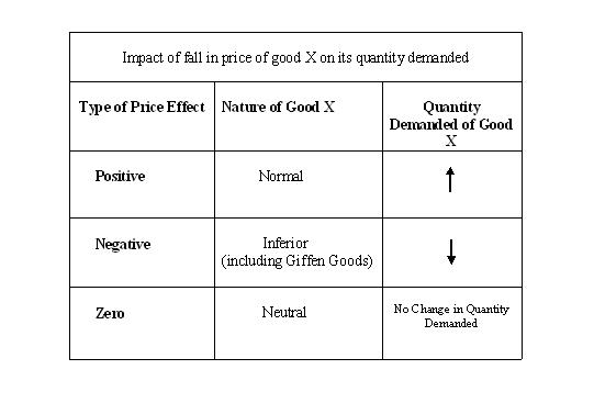
Thus, a price effect is positive in case of normal goods. There is an inverse relationship between price and quantity demanded. It is negative in case of inferior goods (including Giffen goods) where we find a direct relationship between price and quantity demanded. Finally, price effect is zero in case of neutral goods where consumer's quantity demanded is fixed.
Solve the following activity. We then move on to understand positive, negative and zero price effects with the help of indifference curves.
| Positive Price Effect |
In this section we are going to study how the optimal consumption combination changes as a result of change in the price of good X (PX) which is a normal good. Price of Good Y (PY) and consumer's income remaining unchanged. Figure.1 starts with the initial optimal consumption combination attained at point e as discussed in CONSUMER'S EQUILIBRIUM
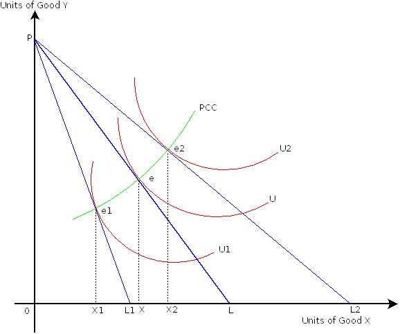
Whenever price of a good representing X-axis change, lower point of the budget constraint shifts as shown in Figure.1.
When the price of good X increases, the budget constraint then becomes steeper, as the lower end point moves leftward. This is shown by budget constraint PL1. The optimal consumption is located at point e1 at which the consumer buys OX1 units of good X. Consumer’s total utility decreases as the optimal consumption combination is located on a lower indifference curve U1.
Similarly, when the price of good X decreases, the budget constraint becomes flatter, as the lower end point moves rightward. This is shown by budget constraint PL2. The optimal consumption is now located at point e2, at which the consumer buys OX2 units of good X. Consumer’s total utility increases as the optimal consumption combination is now located on a higher indifference curve U2.
Chart.2 presents a summary of Figure.1.
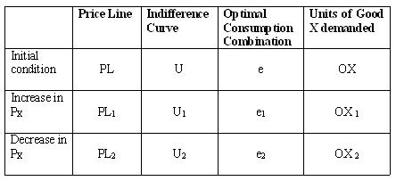
The curve obtained by joining optimal consumption combinations such as e1, e and e2 is called the price consumption curve (PCC). The PCC in Figure.1 is rising upwards to the right. It shows that the consumer successively moves on a higher indifference curve and becomes better off, with a fall in the price of good X (PX).
| Negative Price Effect |
We now study negative price effect. Good X is an inferior good. You will now understand how consumer's optimal consumption combination changes as a result of change in the price of good X (PX) which is an inferior good. Price of good Y (PY) and consumer's income remaining unchanged. Figure.2 starts with the initial optimal consumption combination attained at point e at which OX units of good X are purchased.
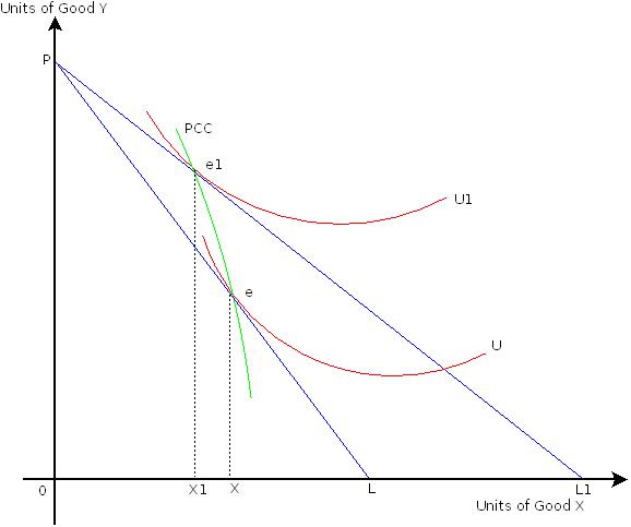
When the price of good X decreases, the budget constraint becomes flatter, as the lower end point moves rightward. This is shown by budget constraint PL1. The optimal consumption is now located at point e1, at which the consumer now buys OX1 units of good X.
Understand that consumer’s total utility has increased as the optimal consumption point is now located on a higher indifference curve U1. The consumer is better-off in terms of total utility. However, she/he reduces consumption of good X to OX1 units as good X is inferior. As mentioned in chart.1 we observe direct relationship between price and quantity demanded of good X.
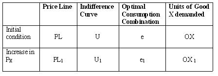
Chart.3 presents a summary of Figure.2.
The pcc obtained by joining optimal consumption combinations such as e, and e1, in Figure.2 rises upwards but bending backwards. It shows that the consumer successively moves on a higher indifference curve and becomes better off, with a fall in the price of good X (PX). She/he is also reducing purchase of good X as it is an inferior good.
| Zero Price Effect |
We now study zero price effect. Good X is a neutral good. You can now see how consumer's optimal consumption combination changes as a result of change in the price of good X (PX) which is a neutral good. Price of good Y (PY) and consumer's income remaining unchanged. Figure.3 starts with the initial optimal consumption combination attained at point e at which OX units of good X are purchased.
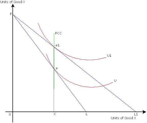
When the price of good X decreases, the budget constraint becomes flatter, as the lower end point moves rightward. This is shown by budget constraint PL1. The optimal consumption is located at point e1, at which the consumer now buys same OX units of good X.
Understand that consumer’s total utility has increased as the optimal consumption point is now located on a higher indifference curve U1. The consumer is better-off in terms of total utility. However, she/he keeps consumption of good X to same OX units as good X is a neutral good. As mentioned in chart.1 we observe no change in quantity demanded of good X.
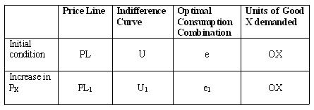
Chart.4 presents a summary of Figure.3.
The pcc obtained by joining optimal consumption combinations such as e, and e1, in Figure.3 is a vertical straight line. It shows that the consumer successively moves on a higher indifference curve and becomes better off, with a fall in the price of good X (PX). She/he is keeping purchase of good X fixed as it is a neutral good.
| Forms of Price Consumption Curve |
In the above discussion on positive, negative and zero price effects we have considered good X to be normal good, inferior good and neutral good respectively. Similarly, we can explain price effect for different types of good Y. Figure.4 shows different forms of PCC for different natures of good X or good Y.
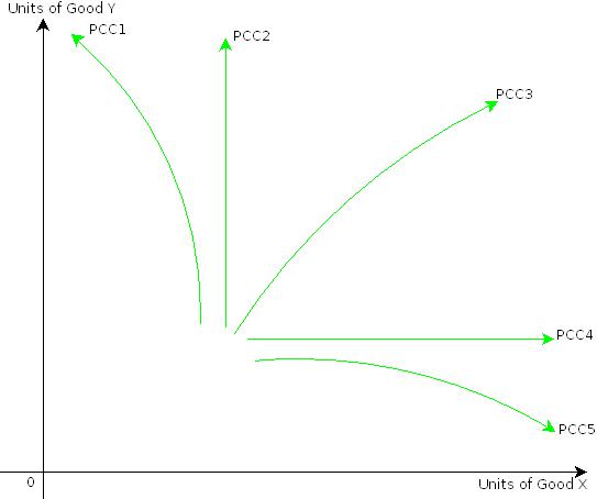
PCC1 is rising upwards and bending towards Y-axis. This form of PCC is obtained when good X is an inferior good (including Giffen goods). The PCC is a vertical straight line as shown by PCC2 when good X is a neutral good. It is a rising curve from left to right as shown by PCC3 when either good X or good Y is a normal good.The PCC is a horizontal straight line as shown by PCC4 when good Y is a neutral good. Finally, PCC5 is rising upwards bending towards X-axis. This form of PCC is obtained when good Y is an inferior good (including Giffen goods). Chart.5 presents a summary of Figure.4.

|
Activity |
| Do you want to see some cartoons on price effect?
Prices of almost all food items in India had soared around June-September 2011. This had affected consumption of basic food items of the people. The cartoon is based on that. [1]
| |

|
Activity |
| Write your activity here | |
| Example: {{{Example}}} |
|

|
Self-Assessment Questions (SAQs) {{{n}}} |
| {{{SAQ}}} | |

|
Results |
People respond to changes in relative prices in order to maximize the utility of spendable income. The price effect represents changes in optimal consumption combination on account of changes in relative prices.
In term of indifference curves, a consumer is better-off when optimal consumption combination is located on a higher indifference curve and vice versa, as a result of relative price changes.
Consumer’s responses to relative price changes vary depending upon the nature of goods. It is positive, negative and zero for normal good, inferior good and neutral good respectively.
These varying responses are important determinants of different forms of market demand curves.

|
Key Terms |

|
Further Readings |
|
|
Global Hunger Index 2011 - The Challenge of Hunger: Taming Price Spikes and Excessive Food Price Volatility
Report
—
Concern Worldwide, Deutsche Welthungerhilfe e. V. (German Agro Action), International Food Policy Research Institute
2011 Global Hunger Index
Fact and Findings: Asia
South Asia has the highest regional 2011 Global Hunger Index (GHI) score—22.6. The 2011 GHI score fell by 25 percent in South Asia compared with its 1990 score, and the 2011 GHI score in Southeast Asia decreased by 44 percent.
The South Asia region reduced its GHI score by more than 6 points between 1990 and 1996—mainly due to a large decline in underweight in children under five, but the fast progress was not maintained. South
Asia has lowered its GHI score by only one point since 2001 despite strong economic growth. Social inequality and the low nutritional, educational, and social status of women, which is a major cause of child under nutrition in the region, have impeded improvements in the GHI score.
Bangladesh and Vietnam saw large gains in improving their GHI score between the 1990 GHI and the 2011 GHI. Vietnam reduced its score by 56 percent, and Bangladesh reduced its score by 36 percent.
In Bangladesh—a country where 25 percent of the population is ultra-poor (living on less than USD $0.50 a day)—only about 7 percent of the population has access to social protection or safety net programs.
The GHI score for North Korea increased by 18 percent since 1990. A weak economy, high military spending, weather-related crop failures, and systematic problems in the agricultural sector have hampered progress.
Cambodia is the only country to improve from an “extremely larming” to “serious” level of hunger since 1990.
Bangladesh, India, and Timor-Leste have the highest prevalence—more than 40 percent—of underweight in children under five.
India ranks below China, Pakistan in Global Hunger Index 2011
ET Bureau Oct 12, 2011, 04.13am IST
Tags:
NEW DELHI: India ranked way below its South Asian neighbours Pakistan, Sri Lanka and China in the global hunger index 2011 released by the International Food Policy and Research Institute. South Asia fared worse than Sub-Saharan Africa netting a score of 22.6 on the global hunger index, or GHI, the report said.
While, India stood 67th amongst 81 countries, Pakistan ranked 59, China ranked fourth, Vietnam ranked 25 and Sri Lanka ranked 36 in the GHI. The report blamed high volatility in food prices for rising hunger levels worldwide.
"The poorest and most vulnerable people bear the heaviest burden when food prices spike or swing unpredictably," said Klaus von Grebmer, lead author of the report and IFPRI Communications Director in the press release.
|- | XXX.5
|
|
- People respond to changes in relative prices in order to maximize the utility of spendable income. The price effect represents changes in optimal consumption combination on account of changes in relative prices.
- In term of indifference curves, a consumer is better-off when optimal consumption combination is located on a higher indifference curve and vice versa, as a result of relative price changes.
- Consumer’s responses to relative price changes vary depending upon the nature of goods. It is positive, negative and zero for normal good, inferior good and neutral good respectively.
- These varying responses are important determinants of different forms of market demand curves.
|- | XXX.6
|
|
Marginal Rate of Substitution: It is the rate at which the consumer is willing to substitute one good for another in consumption.
Price Effect: It represents change in consumer’s optimal consumption combination on account of change in the price of a good and thereby changes in its quantity purchased, price of another good and consumer’s income remaining unchanged.
Positive Price Effect is obtained in case of normal goods. In this case changes in quantity demanded of a good, as a result of price effect, are inversely related to the price change.
Negative Price Effect is obtained in case of inferior goods (including Giffen goods). In this case changes in quantity demanded of a good, as a result of price effect, are directly related to the price change.
Zero Price Effect is obtained in case of neutral goods. In this case there are no changes in quantity demanded of a good as a result of price effect.
|}
Microeconomics, Macroeconomics and Economic Policy
| Essays in Honour of Malcolm Sawyer
Palgrave Macmillan, September 2011ISBN: 978-0-230-29019-8, ISBN10: 0-230-29019-1, 6 1/8 x 9 1/4 inches, 280 pages, 8 b/w tables, 15 figures, |
4 Schaum's Outline of Microeconomics, Fourth Edition (Schaum's Outline Series) [Paperback]
Dominick Salvatore [[Image:]]
Dominick Salvatore (Author)
› Visit Amazon's Dominick Salvatore Page
Find all the books, read about the author, and more.
See search results for this author
Are you an author? Learn about Author Central
(Author)
3.AP Microeconomics Crash Course (Advanced Placement (AP) Crash Course) [Paperback]
David Mayer (Author)
|
α β γ θ Φ Π λ Λ [math]\sqrt{x}[/math] [math]x_{1}^{2}[/math] [math]\sqrt[n]{x}[/math] [math]\sqrt{x^2+y^2}[/math] Fractions [math]\frac{25}{98}[/math]
[math]\sqrt{\frac{x^3+y^3}{x^2+y^2}}[/math] [math]\mathcal{S.I.W.S.COLLEGE}[/math] [math]\mathcal{ANDCOLLEGE}[/math] [math]\sum_{i=0}^{n}x_i=99[/math]
[math]A \rightarrow B[/math] [math]\sum x_i=99[/math] [math]\int x^{2}dx[/math] [math]\int_{0}^{\infty}x^3dx=n[/math]
[math]\frac{dy}{dx}[/math]
[math]x\pm3[/math]
[math]x\geq3[/math] [math]A\subset B[/math]
[math]x\neq3[/math] [math]x\leq3[/math] (![]() : Hi, perhaps you want to read this help link: Help:Latex_Symbol_Tables)
: Hi, perhaps you want to read this help link: Help:Latex_Symbol_Tables)
α
β γ,π,
Λ
Π, λ, Λ
Square root
[math]\sqrt{x^2+y^3}[/math]
[math]\sqrt[n]{x_1^2+y_1^2}[/math]
Fractions
[math]\frac{x^3+z^5}{\sqrt{\omega}}[/math]
[math]\frac{W_m}{W_f}[/math]
[math]\frac{\alpha+\epsilon}{\lambda}[/math]
[math]\frac{\alpha+\epsilon}{\lambda}[/math]
integrals
[math]\int{x^2}dx[/math]
[math]\int_0^4{x^3dx}[/math]
[math]\iint{xydxdy}[/math]
[math]\int_0^\infty\int_0^1xydxdy[/math]
{a'b'c}
differentials
[math]\frac{dy}{dx}[/math]
[math]A\neq{B}[/math]
[math]A\neq B[/math]
[math]A \subset B[/math]
[math]A \rightarrow B[/math], [math]A \uparrow B[/math],[math]A \Leftarrow B[/math]
[math]\bigg \{\frac{W_m}{W_f}\bigg\}^*[/math]
[math]\mathbf{A}\cdot\mathbf{B}[/math], [math]\mathbf{A}\times\mathbf{B}[/math]
calligraphic letters
[math]\mathcal{ANDCOLLEGE}[/math]
[math]\mathcal{A~N~D~COLLEGE}[/math]
[math]\frac{\partial y}{\partial x}[/math]
Matrices
[math]\begin{matrix}0 & 1 & 2\\3 & 4 & 5\end{matrix}[/math]
[math]\begin{pmatrix}0 & 1 & 2\\3 & 4 & 5\end{pmatrix}[/math]
[math]\begin{bmatrix}0 & 1 & 2\\3 & 4 & 5\end{bmatrix}[/math]
[math]\begin{vmatrix}0 & 1 & 2\\3 & 4 & 5\end{vmatrix}[/math]
[math]\begin{Vmatrix}0 & 1 & 2\\3 & 4 & 5\end{Vmatrix}[/math]
[math]\triangle x\triangle p\geq \hbar[/math]
Maths mode accent
[math]\hat{A}[/math], [math]\vec{A}[/math], [math]\bar{A}[/math], [math]\tilde{A}[/math]
[math]\pm2^0C\longleftrightarrow[/math]
F'e3 +
stackrel
[math]A\stackrel{heat}{\longrightarrow}B[/math]
[math]\bar{h}[/math]
[math]\hbar[/math]
[math]\triangle{x}\triangle{p}\geq\hbar[/math]
[math]\nabla^2{x}[/math]
<flash>file=TYBCOM.swf|width=1000|height=500|quality=best</flash>
MICROECONOMICS

|
DECOMPOSITION OF PRICE EFFECT |

|
Introduction |
In the section on price effect we have discussed how a consumer rearranges her/his optimal consumption combination, to once again maximize utility of her/his spendable income, as a response to change in the price of a good. We have also seen consumer's responses to a price change in case of different types of goods.

|
Learning Objectives |
| After reading this chapter, you are expected to learn about: understand 1. 2.
| |
| 1. Meaning of Decomposition of Price Effect |
The price effect is viewed as a combination of income and substitution effects. The substitution effect always works in one direction. A consumer is always induced to buy more units of a cheaper good. Income effect on the other hand could be positive, negative or zero in case of normal, inferior (including Giffen goods) or neutral goods respectively. Refer chart.1 of the section on income effect.
Therefore, the price effect, as the final outcome of the substitution and income effects, depends on their relative direction and magnitude. This is summarized in Chart.1.
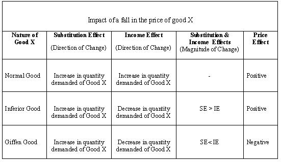
The substitution and income effects work in the same direction when good X is a normal good. The final price effect is then positive. The consumer tends to increase consumption of Good X with fall in its price.
When good X is an inferior good, then the substitution and income effects work in opposite directions. When price of good X (Px)falls, the consumer tends to increase consumption of good X as a result of substitution effect. However, income effect here is negative. The price effect then depends on relative magnitude of the two effects. The final price effect is positive for inferior goods, as change in the consumption of good X as a result of the substitution effect is greater than the income effect.
When good X is a Giffen good then also substitution and income effects work in opposite directions. When price of good X (Px)falls, the consumer tends to increase consumption of good X as a result of substitution effect. However, income effect here is negative. Further, the magnitude of change in units of good X on account of the substitution effect is less than the income effect. The price effect, the final outcome, is therefore negative.
We are now going to study decomposition of the price effect into income and substitution effects with the help of indifference curves.
| 2. Decomposition of Price Effect: Normal Goods |
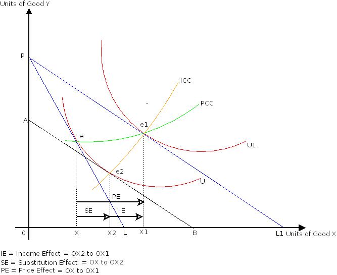
We use the method of compensatory variation in money income in order to decompose the price effect into the income and substitution effects. This is shown in Figure.1. It starts with the initial optimal consumption combination attained at point e
When the price of good X falls, the consumer buys OX1 units of good X at the optimal consumption combination e1 on the budget constraint PL1 and a higher indifference curve U1. The price consumption curve (PCC) obtained by joining points e and e1 rises upwards.
This price effect can be decomposed into the substitution and income effects. This is done by using the method of compensatory variation in consumer's money income. Suppose, we reduce consumer's money income at optimal consumption combination e1 by the amount that is just sufficient to bring her/him back on the initial indifference curve U. This will lead to a downward shift in the budget constraint as shown by budget constraint AB which is parallel to budget constraint PL1. Commodity X is relatively cheaper on budget constraint AB than on PL. e2 is the optimal consumption combination at which the consumer is buying OX2 units of good X. It shows consumer's preference for cheaper good X even after reduction in her/his money income.
Suppose the consumer is given back the money income that was reduced under compensatory variation in her/his money income. The consumer then shifts to optimal consumption combination e1. Thus movement from e2 to e1 represents income effect. Income effect here is positive as good X is a normal good.
Thus, price effect is the net total of substitution effect and income effect. Consumer's movement from optimal consumption combination e to e1, as a result of price effect, can be decomposed into two effects. First the substitution effect, i.e., consumer's movement from e to e2 and then the income effect, i.e., consumer's movement from optimal consumption combination e2 to e1. Thus,
Price Effect = Substitution Effect + Income Effect
In terms of optimal consumption combination:
e to e1 = e to e2 + e2 e1
In terms of units of good X purchased:
XX1 = XX2 + X2 X1
Here, as shown in chart.1, the substitution and income effects are working in same direction. Good X becomes relatively cheaper with fall in its price and the consumer tends to increase its consumption. The income effect is also positive. The consumer tends to increase consumption of good as it is a normal good. This is shown by the Income Consumption Curve (ICC) which is rising upwards The final price effect is, therefore, positive. The consumer finally tends to increase consumption of good X from OX to OX1 with a fall in its price (Px).
| 3. Decomposition of Price Effect: Inferior Goods |
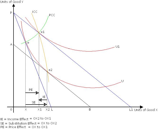
Decomposition of the price effect into substitution and income effects in case of an inferior good is shown in Figure.2 in which good X is an inferior good. It starts with the initial optimal consumption combination attained at point e
When the price of good X falls, the consumer buys OX1 units of good X at the optimal consumption combination e1 on the budget constraint PL1 and a higher indifference curve U1. The price consumption curve (PCC) obtained by joining points e and e1 rises upwards. It shows positive price effect. When price of good X falls the consumer increases consumption of good X from OX to OX1.
Same as section 2, this price effect can be decomposed into the substitution and income effects by using the method of compensatory variation in consumer's money income. Suppose, we reduce consumer's money income at optimal consumption combination point e1 by the amount that is just sufficient to bring her/him back on the initial indifference curve U. This will lead to a downward shift in the budget constraint as shown by budget constraint AB which is parallel to budget constraint PL1. Commodity X is relatively cheaper on budget constraint AB than on PL. e2 is the optimal consumption combination at which the consumer is buying OX2 units of good X. It shows consumer's preference for cheaper good X even after reduction in her/his money income.
Suppose the consumer is given back the money income that was reduced under compensatory variation in her/his money income. The consumer then shifts to optimal consumption combination e1. Thus movement from e2 to e1 represents income effect. Income effect here is negative as good X is an inferior good.
Thus, price effect is the net total of substitution effect and income effect. Consumer's movement from optimal consumption combination e to e1, as a result of price effect, can be decomposed into two effects. First the substitution effect, i.e., consumer's movement from e to e2 and then the income effect, i.e., consumer's movement from optimal consumption combination e2 to e1. Thus,
Price Effect = Substitution Effect + Income Effect
In terms of optimal consumption combination:
e to e1 = e to e2 + e2 e1
In terms of units of good X purchased:
XX1 = XX2 + X2 X1
Here, as shown in chart.1, the substitution and income effects are working in opposite direction. Good X becomes relatively cheaper with fall in its price and the consumer tends to increase its consumption. However the income effect is negative. The consumer tends to reduce consumption of good X as it is an inferior good. This is shown by the Income Consumption Curve (ICC) which is rising upwards but bending backwards. The final price effect is, however, positive as the magnitude of substitution effect is greater than the income effect. The consumer finally tends to increase consumption of good X from OX to OX1 with a fall in its price (Px).
| 4. Decomposition of Price Effect: Giffen Goods |
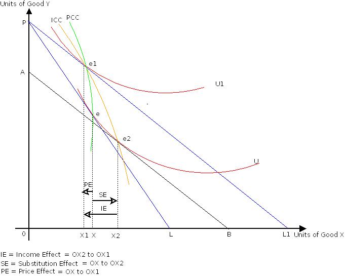
Decomposition of the price effect into substitution and income effects in case of a Giffen good is shown in Figure.3 in which good X is a Giffen good. It starts with the initial optimal consumption combination attained at point e
When the price of good X falls, the consumer buys OX1 units of good X at the optimal consumption combination e1 on the budget constraint PL1 and a higher indifference curve U1. The price consumption curve (PCC) obtained by joining points e and e1 rises upwards but bending backwards towards Y-axis. It shows negative price effect. When price of good X falls the consumer also reduces consumption of good X from OX to OX1.
Same as above, this price effect can be decomposed into the substitution and income effects by using the method of compensatory variation in consumer's money income. Suppose, we reduce consumer's money income at optimal consumption combination point e1 by the amount that is just sufficient to bring her/him back on the initial indifference curve U. This will lead to a downward shift in the budget constraint as shown by budget constraint AB which is parallel to budget constraint PL1. Commodity X is relatively cheaper on budget constraint AB than on PL. e2 is the optimal consumption combination at which the consumer is buying OX2 units of good X. It shows consumer's preference for cheaper good X even after reduction in her/his money income.
Suppose the consumer is given back the money income that was reduced under compensatory variation in her/his money income. The consumer then shifts to optimal consumption combination e1. Thus movement from e2 to e1 represents income effect. Income effect here is negative as good X is a Giffen good.
Thus, price effect is the net total of substitution effect and income effect. Consumer's movement from optimal consumption combination e to e1, as a result of price effect, can be decomposed into two effects. First the substitution effect, i.e., consumer's movement from e to e2 and then the income effect, i.e., consumer's movement from optimal consumption combination e2 to e1. Thus,
Price Effect = Substitution Effect + Income Effect
In terms of optimal consumption combination:
e to e1 = e to e2 + e2 e1
In terms of units of good X purchased:
XX1 = XX2 + X2 X1
Here, as shown in chart.1, the substitution and income effects are working in opposite direction. Good X becomes relatively cheaper with fall in its price and the consumer tends to increase its consumption. However the income effect is negative. The consumer tends to reduce consumption of good X as it is an inferior good. This is shown by the Income Consumption Curve (ICC) which is rising upwards but bending backwards. The final price effect is also negative as the magnitude of substitution effect is less than the income effect. The consumer finally tends to reduce consumption of good X from OX to OX1 with a fall in its price (Px).
DERIVATION OF DEMAND CURVE
MICROECONOMICS

|
DERIVATION OF THE CONSUMER'S DEMAND CURVE |

|
Introduction |
r,,gtv

|
Learning Objectives |
| After reading this chapter, you are expected to learn about: understand 1. 2.
| |
| Derivation of the Consumer's Demand Curve: Normal Goods |
We have already seen how the price consumption curve traces the effect of a change in price of a good on its quantity demanded. However, it does not directly show the relationship between the price of a good and its corresponding quantity demanded. It is the demand curve that shows relationship between price of a good and its quantity demanded. In this section we are going to derive the consumer's demand curve from the price consumption curve . Figure.1 shows derivation of the consumer's demand curve from the price consumption curve where good X is a normal good.
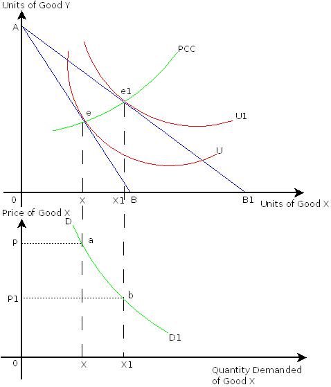
The upper panel of Figure.1 shows price effect where good X is a normal good. AB is the initial price line. Suppose the initial price of good X (Px) is OP. e is the initial optimal consumption combination on indifference curve U. The consumer buys OX units of good X. When price of X (Px)falls, to say OP1, the budget constraint shift to AB1. The optimal consumption combination is e1 on indifference curve U1. The consumer now increases consumption of good X from OX to OX1 units. The Price Consumption Curve (PCC) is rising upwards.
Chart.1 shows the demand relationship derived form the price consumption curve.

The lower panel of Figure.1 shows this price and corresponding quantity demanded of good X as shown in Chart.1. At initial price OP, quantity demanded of good X is OX. This is shown by point a. At a lower price OP1, quantity demanded increases to OX1. This is shown by point b. DD1 is the demand curve obtained by joining points a and b. The demand curve is downward sloping showing inverse relationship between price and quantity demanded as good X is a normal good.
| Derivation of the Consumer's Demand Curve: Giffen Goods |
In this section we are going to derive the consumer's demand curve from the price consumption curve in the case of inferior goods. Figure.2 shows derivation of the consumer's demand curve from the price consumption curve where good X is an inferior good.
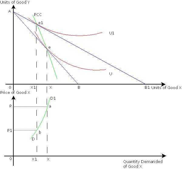
The upper panel of Figure.2 shows price effect where good X is an inferior good. AB is the initial price line. Suppose the initial price of good X (Px)is OP. e is the initial optimal consumption combination on indifference curve U. The consumer buys OX units of good X. When price of X Px) falls, to say OP1, the budget constraint shift to AB1. The optimal consumption combination is e1 on indifference curve U1. The consumer now reduces consumption of good X from OX to OX1 units as good x is inferior. The Price Consumption Curve (PCC) is rising upwards and bending backwards towards the Y-axis.
Chart.1 shows the demand relationship derived form the price consumption curve.

The lower panel of Figure.2 shows this price and corresponding quantity demanded of good X as shown in Chart.2. At initial price OP, quantity demanded of good X is OX. This is shown by point a. At a lower price OP1, quantity demanded decreases to OX1. This is shown by point b. DD1 is the demand curve obtained by joining points a and b. The demand curve is upward sloping showing direct relationship between price and quantity demanded as good X is an inferior good.
| Derivation of the Consumer's Demand Curve: Neutral Goods |
In this section we are going to derive the consumer's demand curve from the price consumption curve in the case of neutral goods. Figure.3 shows derivation of the consumer's demand curve from the price consumption curve where good X is a neutral good.
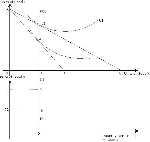
The upper panel of Figure.3 shows price effect where good X is a neutral good. AB is the initial price line. Suppose the initial price of good X (Px) is OP. e is the initial optimal consumption combination on indifference curve U. The consumer buys OX units of good X. When price of X (Px)falls, to say OP1, the budget constraint shift to AB1. The optimal consumption combination is e1 on indifference curve U1 at which the consumer buys same OX units of good X as it is a neutral good. The Price Consumption Curve (PCC) is a vertical straight line.
Chart.3 shows the demand relationship derived form the price consumption curve.

The lower panel of Figure.3 shows this price and corresponding quantity demanded of good X as shown in Chart.3. At initial price OP, quantity demanded of good X is OX. This is shown by point a. At a lower price OP1, quantity demanded remains fixed at OX. This is shown by point b. DD1 is the demand curve obtained by joining points a and b. The demand curve is a vertical straight line showing that the consumption of good X is fixed as good X is a neutral good.
MICROECONOMICS

|
SUBSTITUTION EFFECT
|

|
Introduction |
In the previous section on income effect we have discussed how a consumer rearranges her/his optimal consumption combination, to once again maximize utility of her/his spendable income, as a response to a change in her/his income. We have also seen consumer's responses to income changes in case of different types of goods.

|
Learning Objectives |
| After reading this chapter, you are expected to learn about: understand 1. How consumers arrive at optimal consumption in response to change in relative prices?
| |
| Substitution Effect: Related Concepts |
In this section we are going to study substitution effect. In other words, understand how the optimal consumption combination changes as a result of change in the relative price alone, real income of the consumer remaining unchanged.
We need to understand here the meaning of relative price change and real income remaining unchanged.
In relative price change, comparison is between prices of two goods. For example, between goods X and Y, good X becoms relatively cheaper (costlier) when price of good X (Px)decreases (increases)with price of good Y remaining unchanged.
The real income on the other hand shows purchasing power of the money income. For the given money income, whenever price of a good changes then the purchasing power of consumer's money income increases and so also her/his real income. For example suppose a consumer is spending her/his money income on good X. When the price of the good X decreases, the consumer's purchasing power increases and with same money income she/he is able to purchase more of good X.
Now, a substitution effect shows change in the consumer’s optimal consumption combination on account of change in the relative price alone and thereby changes in her/his quantity purchased of goods X and Y, real income of the consumer remaining unchanged.
Note that consumer's real income changes whenever there is a relative price change. Then, how do we study substitution effect which shows changes in consumer's purchases on account of relative price changes, consumer's real income remaining unchanged?
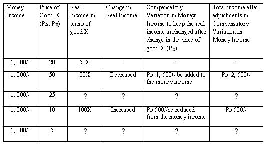
A compensatory variation in money income method is used to neutralize the real income change that takes place on account of the relative price change. The consumer's money income is sufficiently adjusted to compensate her/him for real income changes on account of change in the price of a good.
Solve the following activity to gain adequate clarity on the concepts just discussed, before we move on to understanding substitution effect with the help of indifference curves.
| Hicksian Substitution Effect |
A substitution effect shows change in consumer's optimal consumption combination as a result of change in the relative price alone, real income of the consumer remaining unchanged. Substitution effect is shown in Figure 1. It starts with the initial optimal consumption combination attained at point e at which OX units of good X and OY units of good Y are purchased.
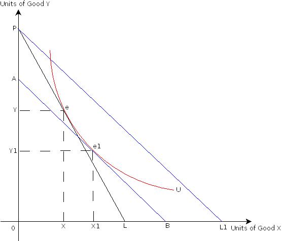
When the price of good X decreases, the budget constraint then becomes flatter, as the lower end point moves rightward. This is shown by budget constraint PL1. The real income of the consumer also increases. This increase in real income will be neutralized through Compensatory Variation in Money Income so that the real income of the consumer remains unchanged. In other words we need to reduce consumer's money income to bring her/him at initial real income level. This adjustment in money income shifts the budget constraint backwards and it is a parallel shift as shown by the price line AB.
The relative prices of goods X and Y are different on budget constraint AB than on the budget constraint PL. Good X is relatively cheaper to good Y on budget constraint PL1 than budget constraint PL. This is because budget constraint PL1 is obtained when the price of good X decreases, price of good Y remaining unchanged. Similarly, good X is relatively cheaper to good Y on budget constraint AB, as it is parallel to PL1.
Thus, good X is relatively cheaper to good Y on budget constraint AB than on budget constraint PL. However, Consumer's real income on budget constraint AB is same as her/his real income on budget constraint PL, as budget constraint AB is obtained through compensatory variation in consumer's money income.
Figure.1 shows that on the new budget constraint AB, obtained after compensatory variation in money income, the consumer attains optimal consumption combination at point e1 which is on the same indifference curve U and purchases OX1 units of good X and OY1 units of good Y.
Thus, consumer's movement from optimal consumption combination e to e1 shows substitution effect. Similarly, increase in her/his consumption of good X by XX1 and decrease in consumption of good Y by YY1 is on account of change in the relative price alone, real income of the consumer remaining unchanged.
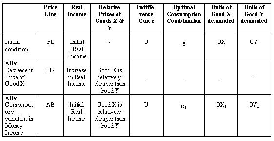
Thus a substituion effect shows consumers preference for relatively cheaper goods. In the case of a substitution effect the consumer remains on the same indifference curve. Chart 1 presents a summary of Figure.1.
| Slutsky Substitution Effect |


