INDIFFERENCE CURVES: DECOMPOSITION OF PRICE EFFECT
MICROECONOMICS

|
DECOMPOSITION OF PRICE EFFECT |

|
Introduction |
In the section on price effect we have discussed how a consumer rearranges her/his optimal consumption combination, to once again maximize utility of her/his spendable income, as a response to change in the price of a good. We have also seen consumer's responses to a price change in case of different types of goods.

|
Learning Objectives |
| After reading this chapter, you are expected to learn about: understand 1. 2.
| |
| 1. Meaning of Decomposition of Price Effect |
The price effect is viewed as a combination of income and substitution effects. The substitution effect always works in one direction. A consumer is always induced to buy more units of a cheaper good. Income effect on the other hand could be positive, negative or zero in case of normal, inferior (including Giffen goods) or neutral goods respectively. Refer chart.1 of the section on income effect.
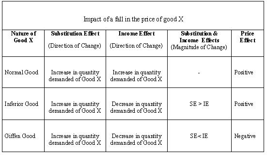
Therefore, the price effect, as the final outcome of the substitution and income effects, depends on their relative direction and magnitude. This is summarized in Chart.1.

The substitution and income effects work in the same direction when good X is a normal good. The final price effect is then positive. The consumer tends to increase consumption of Good X with fall in its price.
When good X is an inferior good, then the substitution and income effects work in opposite directions. When price of good X (Px)falls, the consumer tends to increase consumption of good X as a result of substitution effect. However, income effect here is negative. The price effect then depends on relative magnitude of the two effects. The final price effect is positive for inferior goods, as change in the consumption of good X as a result of the substitution effect is greater than the income effect.
When good X is a Giffen good then also substitution and income effects work in opposite directions. When price of good X (Px)falls, the consumer tends to increase consumption of good X as a result of substitution effect. However, income effect here is negative. Further, the magnitude of change in units of good X on account of the substitution effect is less than the income effect. The price effect, the final outcome, is therefore negative.
We are now going to study decomposition of the price effect into income and substitution effects with the help of indifference curves.
| 2. Decomposition of Price Effect: Normal Goods |
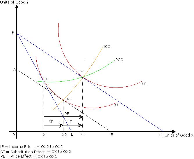
We use the method of compensatory variation in money income in order to decompose the price effect into the income and substitution effects. This is shown in Figure.1. It starts with the initial optimal consumption combination attained at point e
When the price of good X falls, the consumer buys OX1 units of good X at the optimal consumption combination e1 on the budget constraint PL1 and a higher indifference curve U1. The price consumption curve (PCC) obtained by joining points e and e1 rises upwards.
This price effect can be decomposed into the substitution and income effects. This is done by using the method of compensatory variation in consumer's money income. Suppose, we reduce consumer's money income at optimal consumption combination e1 by the amount that is just sufficient to bring her/him back on the initial indifference curve U. This will lead to a downward shift in the budget constraint as shown by budget constraint AB which is parallel to budget constraint PL1. Commodity X is relatively cheaper on budget constraint AB than on PL. e2 is the optimal consumption combination at which the consumer is buying OX2 units of good X. It shows consumer's preference for cheaper good X even after reduction in her/his money income.
Suppose the consumer is given back the money income that was reduced under compensatory variation in her/his money income. The consumer then shifts to optimal consumption combination e1. Thus movement from e2 to e1 represents income effect. Income effect here is positive as good X is a normal good.
Thus, price effect is the net total of substitution effect and income effect. Consumer's movement from optimal consumption combination e to e1, as a result of price effect, can be decomposed into two effects. First the substitution effect, i.e., consumer's movement from e to e2 and then the income effect, i.e., consumer's movement from optimal consumption combination e2 to e1. Thus,
Price Effect = Substitution Effect + Income Effect
In terms of optimal consumption combination:
e to e1 = e to e2 + e2 e1
In terms of units of good X purchased:
XX1 = XX2 + X2 X1
Here, as shown in chart.1, the substitution and income effects are working in same direction. Good X becomes relatively cheaper with fall in its price and the consumer tends to increase its consumption. The income effect is also positive. The consumer tends to increase consumption of good as it is a normal good. This is shown by the Income Consumption Curve (ICC) which is rising upwards The final price effect is, therefore, positive. The consumer finally tends to increase consumption of good X from OX to OX1 with a fall in its price (Px).
| 3. Decomposition of Price Effect: Inferior Goods |
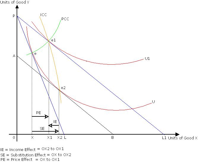
Decomposition of the price effect into substitution and income effects in case of an inferior good is shown in Figure.2 in which good X is an inferior good. It starts with the initial optimal consumption combination attained at point e
When the price of good X falls, the consumer buys OX1 units of good X at the optimal consumption combination e1 on the budget constraint PL1 and a higher indifference curve U1. The price consumption curve (PCC) obtained by joining points e and e1 rises upwards. It shows positive price effect. When price of good X falls the consumer increases consumption of good X from OX to OX1.
Same as section 2, this price effect can be decomposed into the substitution and income effects by using the method of compensatory variation in consumer's money income. Suppose, we reduce consumer's money income at optimal consumption combination point e1 by the amount that is just sufficient to bring her/him back on the initial indifference curve U. This will lead to a downward shift in the budget constraint as shown by budget constraint AB which is parallel to budget constraint PL1. Commodity X is relatively cheaper on budget constraint AB than on PL. e2 is the optimal consumption combination at which the consumer is buying OX2 units of good X. It shows consumer's preference for cheaper good X even after reduction in her/his money income.
Suppose the consumer is given back the money income that was reduced under compensatory variation in her/his money income. The consumer then shifts to optimal consumption combination e1. Thus movement from e2 to e1 represents income effect. Income effect here is negative as good X is an inferior good.
Thus, price effect is the net total of substitution effect and income effect. Consumer's movement from optimal consumption combination e to e1, as a result of price effect, can be decomposed into two effects. First the substitution effect, i.e., consumer's movement from e to e2 and then the income effect, i.e., consumer's movement from optimal consumption combination e2 to e1. Thus,
Price Effect = Substitution Effect + Income Effect
In terms of optimal consumption combination:
e to e1 = e to e2 + e2 e1
In terms of units of good X purchased:
XX1 = XX2 + X2 X1
Here, as shown in chart.1, the substitution and income effects are working in opposite direction. Good X becomes relatively cheaper with fall in its price and the consumer tends to increase its consumption. However the income effect is negative. The consumer tends to reduce consumption of good X as it is an inferior good. This is shown by the Income Consumption Curve (ICC) which is rising upwards but bending backwards. The final price effect is, however, positive as the magnitude of substitution effect is greater than the income effect. The consumer finally tends to increase consumption of good X from OX to OX1 with a fall in its price (Px).
| 4. Decomposition of Price Effect: Giffen Goods |
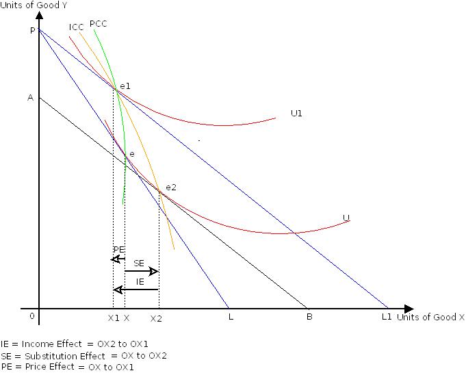
Decomposition of the price effect into substitution and income effects in case of a Giffen good is shown in Figure.3 in which good X is a Giffen good. It starts with the initial optimal consumption combination attained at point e
When the price of good X falls, the consumer buys OX1 units of good X at the optimal consumption combination e1 on the budget constraint PL1 and a higher indifference curve U1. The price consumption curve (PCC) obtained by joining points e and e1 rises upwards but bending backwards towards Y-axis. It shows negative price effect. When price of good X falls the consumer also reduces consumption of good X from OX to OX1.
Same as above, this price effect can be decomposed into the substitution and income effects by using the method of compensatory variation in consumer's money income. Suppose, we reduce consumer's money income at optimal consumption combination point e1 by the amount that is just sufficient to bring her/him back on the initial indifference curve U. This will lead to a downward shift in the budget constraint as shown by budget constraint AB which is parallel to budget constraint PL1. Commodity X is relatively cheaper on budget constraint AB than on PL. e2 is the optimal consumption combination at which the consumer is buying OX2 units of good X. It shows consumer's preference for cheaper good X even after reduction in her/his money income.
Suppose the consumer is given back the money income that was reduced under compensatory variation in her/his money income. The consumer then shifts to optimal consumption combination e1. Thus movement from e2 to e1 represents income effect. Income effect here is negative as good X is a Giffen good.
Thus, price effect is the net total of substitution effect and income effect. Consumer's movement from optimal consumption combination e to e1, as a result of price effect, can be decomposed into two effects. First the substitution effect, i.e., consumer's movement from e to e2 and then the income effect, i.e., consumer's movement from optimal consumption combination e2 to e1. Thus,
Price Effect = Substitution Effect + Income Effect
In terms of optimal consumption combination:
e to e1 = e to e2 + e2 e1
In terms of units of good X purchased:
XX1 = XX2 + X2 X1
Here, as shown in chart.1, the substitution and income effects are working in opposite direction. Good X becomes relatively cheaper with fall in its price and the consumer tends to increase its consumption. However the income effect is negative. The consumer tends to reduce consumption of good X as it is an inferior good. This is shown by the Income Consumption Curve (ICC) which is rising upwards but bending backwards. The final price effect is also negative as the magnitude of substitution effect is less than the income effect. The consumer finally tends to reduce consumption of good X from OX to OX1 with a fall in its price (Px).


