SUBSTITUTION EFFECT/Next
| Hicksian Substitution Effect |
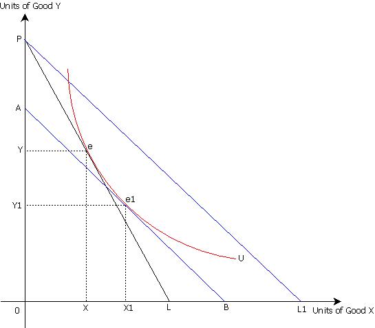
A substitution effect shows change in consumer's optimal consumption combination as a result of change in the relative price alone, real income of the consumer remaining unchanged. Substitution effect is shown in Figure 1. It starts with the initial optimal consumption combination attained at point e at which OX units of good X and OY units of good Y are purchased.

When the price of good X decreases, the budget constraint then becomes flatter, as the lower end point moves rightward. This is shown by budget constraint PL1. The real income of the consumer also increases. This increase in real income will be neutralized through Compensatory Variation in Money Income so that the real income of the consumer remains unchanged. In other words we need to reduce consumer's money income to bring her/him at initial real income level. This adjustment in money income shifts the budget constraint backwards and it is a parallel shift as shown by the price line AB.
The relative prices of goods X and Y are different on budget constraint AB than on the budget constraint PL. Good X is relatively cheaper to good Y on budget constraint PL1 than budget constraint PL. This is because budget constraint PL1 is obtained when the price of good X (Px) decreases, price of good Y (Py)remaining unchanged. Similarly, good X is relatively cheaper to good Y on budget constraint AB, as it is parallel to PL1.
Thus, good X is relatively cheaper to good Y on budget constraint AB than on budget constraint PL. However, Consumer's real income on budget constraint AB is same as her/his real income on budget constraint PL, as budget constraint AB is obtained through compensatory variation in consumer's money income.
Figure.1 shows that on the new budget constraint AB, obtained after compensatory variation in money income, the consumer attains optimal consumption combination at point e1 which is on the same indifference curve U and purchases OX1 units of good X and OY1 units of good Y.
Thus, consumer's movement from optimal consumption combination e to e1 shows substitution effect. Similarly, increase in her/his consumption of good X by XX1 and decrease in consumption of good Y by YY1 is on account of change in the relative price alone, real income of the consumer remaining unchanged.
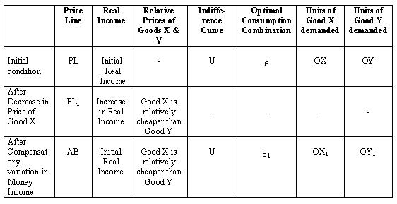
Thus a substituion effect shows consumers preference for relatively cheaper goods. In that sense the substitution effect works in opposite direction. It is always negative. A consumer buys more units of a good whose price is relatively lower. Further, the consumer remains on the same indifference curve. Chart 1 presents a summary of Figure.1.

| Slutsky's Substitution Effect |
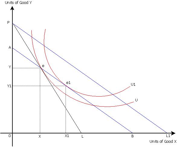
Slutsky's substituion effect approach differers from the Hicksian approach in terms of compensatory variation in money income. In Hicksian approach the compensatory variation in money income is to the extent that would bring the consumer back at initial income level (utility level) or on the original indifference curve. On the other hand, in Slutsky's substitution effect approach the compensatory variation in money income is to the extent to bring the consumer back to the original optimal consumption combination. This is shown in Figure 2. It starts with the initial optimal consumption combination attained at point e at which OX units of good X and OY units of good Y are purchased.

When the price of good X decreases, the budget constraint becomes flatter, as shown by budget constraint PL1 . The real income of the consumer also increases. This increase in real income is neutralized through Compensatory Variation in Money Income so that the consumer is able to buy the initial optimal consumption combination e. This adjustment in money income shifts the budget constraint backwards and it is a parallel shift as shown by the budget constraint AB which passes through point e.
The relative prices of goods X and Y are different on budget constraint AB than on the budget constraint PL. Good X is relatively cheaper to good Y on budget constraint PL1 than budget constraint PL. This is because budget constraint PL1 is obtained when the price of good X (Px) decreases, price of good Y (Py)remaining unchanged. Similarly, good X is relatively cheaper to good Y on budget constraint AB, as it is paralle to PL1.
Thus, good X is relatively cheaper to good Y on budget constraint AB than on budget constraint PL. Figure.2 shows that on the new budget constraint AB, the consumer attains optimal consumption combination at point e1 which is on a higher indifference curve U1 and purchases OX1 units of good X and OY1 units of good Y.
Thus, consumer's movement from optimal consumption combination e to e1 shows substitution effect. Similarly, increase in her/his consumption of good X by XX1 and decrease in consumption of good Y by YY1 is on account of change in the relative price alone, real income of the consumer remaining unchanged. However, unlike in Hicksian approach, the consumer is now at higher utility levels as combination e1 is on a higher indifference curve U1.
| Comparision of Hicksian and Slutsky's Substitution Effect approach |
The above discussion shows that the basic difference between the two approaches arises in terms of how much money income variation is essential for real income to remain unchanged. There is no general reason to prefer one approach over the other. The two approaches are dealing with different set of questions. In the Hicksian approach, income compensation is to the extent to bring the consumer back on the original level of utility or well-being. The consumer is neighter better off nor worse off. This concept of money compensation is useful for welfare comparisons.
In Slutsky's approach the compensatory variation in money income is to the extent to bring the consumer back to the initial optimal consumption combination. The variables such as income, price changes and initial consumption combination are observable and therefore easy to calculate.
For further details refer [1]
