GSE Stat Methods I - Review Notes

Project to Create Statistics Content Modules
Project	StatisticsContent
Design	Objectives  |  Learning Design
Resources	Reading in statistics  |  By type  |  By topic
Content	Learn by doing
Intro Stats course	Syllabus  |  Online course schedule  |  Schedule for in-person meetings  |  Plans for in-person meetings
GSE Stat Methods II	Review notes  |  Topic resources

The following review is based on the indicated chapter and section of

Moore, D. S., McCabe, G. P., & Craig, B. A. (2012). Introduction to the practice of statistics (7th ed). New York: W. H. Freeman.

The questions and items for display are organized as a slide show. The sub-bullets for each point support discussion and content to be written out on the board.

Tests of Significance (6.2)

• Consider a situation where a student is brought before an academic committee with a claim that she cheated. The committee assumes that the student is innocent until proven guilty. The instructor presents convincing evidence of cheating. What should the committee decide as to whether or not the student cheated?
  • committee should find evidence convincing and decide that student cheated.
• Tests of significance work similarly. Identify the following in the cheating story.

1. Identify two opposing claims
   • student claims innocence (claim 1); instructor claims she cheated (claim 2).
   • claim 1 is challenged by claim 2
   • begin with assumption that claim 1 is true.
2. Collect evidence
   • instructor provides evidence against claim 1
   • observations in sample will serve as evidence against claim 1
3. Assess evidence
   • committee evaluates evidence: how likely (probability based) to observe this evidence if student is innocent
   • evaluate sample statistics in context of sampling distribution; determine how likely to observe this result if it were to have occurred by chance.
4. Make a decision
   • If very unlikely that student could be innocent (claim 1) given evidence (strong evidence against claim 1), then reject claim 1 and decide for claim 2
   • If likely that student could be innocent (claim 1) given evidence (weak evidence against claim 1), then stay with claim 1 (cannot reject claim 1 in favor of claim 2). Note: we do not say we accept claim one, we just don't have anything better to conclude.

• What do we call the two claims in tests of significance?
  • Null hypothesis (H_o), claim 1
    • typically statement of no effect, no difference; the assumed usual state
  • Alternative hypothesis (H_a), claim 2
    • statement that disagrees with H_o, specifying what we think might be going on; written as an "opposite" of null hypothesis.
  • also called hypothesis testing
• Example: Traditional practice suggests that college students should study 2 hours for every 1 hour of classroom time. Using this rule, a student with 15 hours of classroom time per week (i.e., 15 credit hours, denoted full-time) should study on average 30 hours per week. A researcher is interested in whether this rule applies at Rutgers University. What are the null and alternative hypotheses for this study? (Step 1)
  • H₀: The average time full-time Rutgers students study outside of class is 30 hours per week.
  • H_a: The average time full-time Rutgers students study outside of class is not 30 hours per week.
• When wording the hypotheses (claims) who are they about?
  • the population
  • the population in our example is the university students
• If we suspected that full-time Rutgers students study less than 30 hours per week, how would we have stated H_a?
  • H_a: The average time full-time Rutgers students study outside of class is less than 30 hours per week.
  • One-sided alternative, could be greater than or less than
  • Two-sided alternative, population could differ in either direction.
  • Must have a specific direction firmly in mind (without looking at the data) to choose one-sided
• Example (continued): The researcher obtains a random sample of 50 college students currently taking 15 credits and collects the number of hours they study per week: x-bar = 27 and sd = 5 hours per week. What evidence was collected? How might we summarize the evidence against H₀? (Step 2)
  • evidence is the sample mean and sd.
  • we can compare the sample results to the hypothesized value
• For this example, we will employ a z statistic to compare the sample mean to the hypothesized value. How does this work? What do we call this type of statistic, generally speaking?
  • [math]z = \frac{estimate - hypothesized\ value}{standard\ deviation\ of\ the\ estimate} = \frac{28 - 30}{.7} = -2.86[/math]
  • assume standard deviation of estimate is .7
  • called a test statistic....this is a very typical form
• To assess the evidence we ask the question: how likely is it to get data like that observed when H₀ is true? What do we need to answer this question? (Step 3)
  • the probability of obtaining this value or one more extreme, if the population parameter in H₀ is true.
  • called the p-value
  • if very small, then unlikely to observe this value or one more extreme if H₀ is true.
  • if large, then not surprising to see a value like this, if H₀ is true. Could have happened by chance
• What can we use to give us this probability....of observing a particular value or one more extreme given the population parameter provided in H₀.
  • sampling distribution (ask if it is safe to use the sampling distribution of the mean for this example.....yes, n>40)
  • (draw sampling distribution of x-bar for μ=30, σ=.7)
  • the z-statistic, -2.86, is from a Normal distribution representing the sampling distribution of the mean.
  • (draw Normal distribution, shade areas outside +/-2.86)
  • for a two sided H_a, P(Z <= -2.86 or Z >= 2.86)...sum the lower and upper tails: .0021*2=.0042
• A p-value of p=.0042 is pretty small, but is it small enough to decide against H₀ (that the population mean is 30)? How can we decide? (Step 4)
  • compare our result to a threshold value
  • pre-determined
  • called significance level, α.
• What are some common significance levels? What do they mean?
  • α=.05, α=.01, α=.1
  • if we find a result that would occur less than 5% (1%, 10%) of the time, when H₀ is true, then we decide to reject H₀ and accept H_a.
  • our result is statistically significant at level α.
• What do we conclude if the p value is not smaller than α?
  • we decide that our data do not provide enough evidence to reject Ho
  • we can also say that the data do not provide enough evidence to accept Ha.
  • we cannot say that the data support H₀, or that we accept H₀.
• What do we conclude in our example for p=.0042?

  H₀: The average time full-time Rutgers students study outside of class is 30 hours per week.

  H_a: The average time full-time Rutgers students study outside of class is not 30 hours per week.

  assume we set α=.05 before the data were collected

  p=.0042

  • our result is statistically significant
  • we reject H₀ and conclude that the average time full-time Rutgers students study outside of class is not 30 hours per week.
• What if before we collected the data we suspected that Rutgers students, on average, study less than 30 hours per week. How does this change how we assess the evidence and what we conclude?
  • (draw Normal distribution with z=-2.86 and shade only area below)
  • our p-value is smaller....p=.0021....more powerful test because we have prior information about direction of difference
  • our conclusion doesn't change.
• Example: In 2011, the SAT Critical Reading (SAT-CR) test had a mean of 496 and a standard deviation of 114. As XYZ College has a liberal arts focus, the academic dean suspects that XYZ students score higher than the national average. A random sample of 40 XYZ students had an average SAT-CR score of 522. Assume that the population standard deviation is the standard deviation of scores at XYZ College. Does the sample data support the dean's claim that XYZ College students have a higher average score?
  • (draw the population, with sample n=40 removed, label)
• Step 1: What are the null and alternative hypotheses? What significance level should we use?

  • H₀: μ=486; The average SAT-CR score for students at XYZ College is 496.

    H_a: μ>486; The average SAT-CR score for students at XYZ College is greater than 496.

  • α=.05
• Step 2: What is the evidence against H₀?
  • sampling distribution? x-bar
  • is it safe to use the distribution to determine area under the curve? yes n=40
  • test statistic? [math]z = \frac{estimate - hypothesized\ value}{standard\ deviation\ of\ the\ estimate}[/math]
  • x-bar = 522
  • the sd for the sampling distribution of x-bar is σ/√n = 114/√40 = 18
  • [math]z = \frac{\bar{x} - \mu_0}{\sigma_\bar{x}} = \frac{522 - 496}{18} = 1.44[/math]
• Step 3: What is the probability of obtaining a sample result this extreme or more extreme, if H₀ is true (if mean of SAT-CR for XYZ College students is 496)?
  • (draw Normal distribution, label z=1.44, shade area above)
  • P(Z > 1.44) = .075
  • p=.075
• Step 4: What do we conclude?
  • p=.075 is not less than α=.05, we fail to reject H₀
  • there is not enough evidence to conclude that the mean SAT-CR score at XYZ College is greater than 496.
• We have just performed a particular test of significance. What is this test called?
  • z test for a population mean
  • with known population standard deviation σ

Estimating with Confidence (6.1)

• What is the best estimate of the population mean, μ? Why?
  • the sample mean, x-bar, of a random sample is an unbiased estimate of μ.
  • law of large numbers says that as the sample size increases, x-bar will approach value of μ.
• What can we use to help us better understand the possible values of x-bar?
  • sampling distribution of x-bar.
  • shows the variability
• Example: Suppose you want to know the average height of undergraduate women at Rutgers. We know that the standard deviation of heights of young women in the US is 2.5. We obtain a random sample of 100 women currently enrolled as undergraduates at Rutgers. Their mean height is 64.8 inches with a standard deviation of 2.7 inches. What do we know about x-bar, the mean height of Rutgers undergraduate women?
  • CLT says the sampling distribution is N(μ, σ/√n) = N(μ, .25)...σ/√n = 2.5/10 = .25
  • draw and label distribution
  • note: not sd for Rutgers undergrad women; in most cases we will not know the population standard deviation
• How might we construct a 95% confidence interval for the mean of this distribution?
  • use the standard deviation rule for 95%
  • draw +/- 2 standard deviations (μ - .50, μ + .50) onto the distribution
  • 95% chance that x-bar occurs between μ - .50, μ + .50
  • as the distance between x-bar and μ is the same from either direction, we can flip this statement to say
    • we are 95% confident that the true population parameter, μ, falls within the interval [math]\bar{x} - .50[/math] and [math]\bar{x} + .50[/math]
    • in context: we are 95% confident that the average height of Rutgers undergraduate women is between 64.3 inches and 65.3 inches
    • of course our method could be wrong...which we estimate to be the case 5% of the time.
• What name do we use to refer to the value .50 in our example?
  • margin of error
  • quantifies the variability of the estimate in relation to our level of confidence
  • for 95% confidence margin of error approx= 2*(σ/√n)
• What is the general form for a confidence interval?
  • estimate +/- margin of error
  • for a sample mean....[math]\bar{x} \pm 2*(\sigma/ \sqrt{n})[/math]
  • example, we are 95% confident that the average height of Rutgers undergraduate women is 64.8 +/- .5 inches.
• How does the following image support "the population parameter, μ, must be within roughly 2 standard deviations from the sample average, x-bar, in 95% of all samples."
  • (display image of confidence intervals for a sample of x-bars...from text)
  • out of the 25 confidence intervals displayed, only one range does not include μ.
• Using the standard deviation rule, we said the general form of the confidence interval for the population mean is [math]\bar{x} \pm 2*(\sigma/√n)[/math]. How can we make this more precise?
  • note that there is a 95% chance that a Normal random variable will take a value within 1.96 standard deviations of its mean.
  • z-score = +/-1.96 bounds the middle 95%.
  • [math]\bar{x} \pm 1.96*(\sigma/√n)[/math]
• How do we adjust the method if we want to be 99% confident or 90% confident?
  • C is used to indicate the confidence level: C=.90, C=.95, C=.99
  • adjust the margin of error to be larger or smaller...to be more or less confident
  • (display image of N dist, show C% under Normal curve, with +/- margin of error)
• What are the values which bound the middle 99% and 90% of the distribution of x-bar?
  • the corresponding z-score * σ/√n
  • z-score for .90 = 1.645, z-score for .99 = 2.576
• The heights of Rutgers undergraduate women has an unknown mean (μ) and known standard deviation σ = 2.5. A simple random sample of 100 women is found to have a sample mean height x-bar=64.8. Estimate μ with a 90%, 95%, and 99% confidence interval.
  • 90%: [math]\bar{x} \pm 1.645 * \frac{\sigma}{\sqrt{n}} = 64.8 \pm 1.645 \frac{2.5}{\sqrt{100}} = 64.8 \pm .41 = (64.39, 65.21)[/math]
  • 95%: [math]\bar{x} \pm 1.960 * \frac{\sigma}{\sqrt{n}} = 64.8 \pm 1.960 \frac{2.5}{\sqrt{100}} = 64.8 \pm .49 = (64.31, 65.29)[/math]
  • 99%: [math]\bar{x} \pm 2.576 * \frac{\sigma}{\sqrt{n}} = 64.8 \pm 2.576 \frac{2.5}{\sqrt{100}} = 64.8 \pm .64 = (64.16, 65.44)[/math]
• What do we notice about the size of these intervals?
  • (draw them on a normal distribution with mean 64.8)
  • the more confident, the wider the interval for μ...the less precise the estimate
  • There is a trade-off between the level of confidence and the precision with which the parameter is estimated.
• What are the general formulas for the confidence interval and the margin of error?
  • [math]\bar{x} \pm z^* * \frac{\sigma}{\sqrt{n}}[/math]
    • z* is the +/- z-score which bounds the middle C% of Normal dist
    • (label z* as confidence multiplier and σ/√n as st. dev. of estimate)
  • [math]\bar{x} \pm m[/math]
  • estimate +/- margin of error
  • (draw line with m in each direction of estimate...confidence interval is length 2m
  • m tells us how precise the confidence interval is....the estimate tells us the location
• How can we use m to make the confidence interval more precise? m = z*(σ/√n)
  • a larger n will result in a smaller margin of error
• How is the margin of error impacted if we increase the sample size of Rutgers undergraduate women to 400. x-bar = 64.8, population standard deviation σ = 2.5, 95% confidence for n=100 is (64.31, 65.29)
  • 95%: [math]\bar{x} \pm 1.960 * \frac{\sigma}{\sqrt{n}} = 64.8 \pm 1.960 \frac{2.5}{\sqrt{400}} = 64.8 \pm .28 = (64.52, 65.08)[/math]
  • a sampling distribution of X-bar based on larger sample size has a smaller SD...less spread out.
  • larger sample size means we are more confident in our estimate being close to μ.
  • sometimes a larger sample size is too costly, or simply not available.
• An educational researcher is interested in estimating μ, the mean score on the math part of the SAT (SAT-M) of all community college students in his state with a margin of error of 5, at the 95% confidence level. What is the sample size needed to achieve this? (σ is assumed to be 100).
  • [math]m = z^* * \frac{\sigma}{\sqrt{n}} = 2 * \frac{100}{\sqrt{n}} = 5[/math]
  • [math]\sqrt{n} = \frac{2*100}{5}[/math]
  • [math]n = \left ( \frac{2*100}{5} \right )^2 = 1600[/math]
  • generally speaking, [math]n = \left ( \frac{z^* * \sigma}{m} \right )^2[/math]
• If the answer were 1600.2, how would you decide what n to use?
  • round up to next person to be more conservative....larger sample will get you slightly smaller m
• What is the most important requirement underpinning the accuracy of confidence intervals?
  • the data is a random sample from the population....for this method the data must be a SRS
  • the margin of "error" includes only random sampling error....the differences between one random sample and another.

Introduction to inference (intro)

• What is statistical inference?
  • Display OLI big picture image
  • inferring something about the population based on what is measured in the sample
• What role does probability play in statistical inference?
  • tells us what might happen by chance alone
• What role does a sampling distribution play in statistical inference?
  • gives us information about the variability of samples, if we were to use the inference method many times
  • more theoretical than practical as we rarely know the truth about a population
• What requirement must underlie the sampling distribution for us to safely use it for making statistical inference?
  • The data come from a random sample or a randomized experiment
• In a recent poll of a random sample of 1,200 undergraduates, the average amount of time spent on the internet was 19 hours per week. We are 95% confident that μ, the mean amount of time U.S. undergraduates spent on the internet per week, is between 18.36 hours and 19.64 hours. What do we call this type of interval?
  • confidence interval....95% confident
  • any thoughts on how this works?
• It was claimed that among all U.S. adults, about half are in favor of instituting national standards in K-12 schools and about half are against it. In a recent poll of a random sample of 1,200 U.S. adults, 40% were in favor of instituting national standards. This data, therefore, provides some evidence against the claim. What statistical method is employed in this statement?
  • test of significance
  • hypothesis testing
  • any thoughts on how this works?

Sampling distributions for counts and percents (5.2)

• A survey of 100 high school students randomly selected from the NYC school district asked the following. What is the difference between these two random variables:
  • How many minutes of study hall did you have today? (X)....quantitative, continuous
    • useful to calculate the sample mean
  • did you buy food in you school's cafeteria today? (Y)....categorical, discrete
    • useful to calculate the count of yes's (or no's)
    • counts are a common variable in statistics
• The shape of the sampling distribution of sample means is Normal. What is the shape of the sampling distribution of counts?
  • Binomial
  • we will not be discussing the specifics of this distribution, but if you are going on in statistics, suggest studying this distribution.
• What else do we often report along with an overall count, which helps us interpret the meaning of the count?
  • sample proportion [math]\hat{p} = \frac{Y}{n}[/math]
  • Let's say that Y = 56....p-hat = 56/100 = .56
  • if we had a different sample size, we would get a different p-hat.
• What does the sampling distribution of p-hat look like?
  • eg, the distribution of all possible p-hats calculated from all possible 100 student samples from the NYC high schools.
  • (display sampling distributions for n=100 and n=2500 from ips7e, chapt 3.3)
  • center: mean of p-hats should equal population proportion, p
  • spread: the larger the n, the less spread out the possible p-hats around p
  • shape: appears Normal
  • in fact the sample proportion is a special case of the mean.....the mean of the data if coded 1 and 0.
• What is the mean of the sampling distribution of the sample proportion?
  • [math]\mu_\hat{p} = p[/math]
• What is the standard deviation of the sampling distribution of the sample proportion?
  • [math]\sigma_\hat{p} = \sqrt{ \frac{p(1-p)}{n}}[/math]
  • in fact this formula doesn't work quite right when sample is SRS
  • good approximation when population is 20 times larger than sample.
• What can we say about p-hat as it relates to its estimation of p?
  • p-hat is an ubiased estimate of p
• How does the formula for sigma p-hat confirm that the variability will decrease as the sample size increases?
  • sample size is in the denominator....as it gets bigger, [math]\sigma_\hat{p}[/math] gets smaller
• If the sample proportion is in fact a mean, what can we use to support the idea that the sampling distribution of the sample proportion is Normal?
  • the central limit theorem says that p-hat is approximately Normal when the sample size is large
  • [math]\hat{p} \sim N \left ( p, \sqrt{\frac{p(1-p)}{n}} \right )[/math]
  • draw Normal distribution and label [math]\mu = p[/math], and [math]\sigma = \sqrt{\frac{p(1-p)}{n}}[/math]
• How large does the sample size need to be in order for p-hat to be Normally distributed?
  • this is the case when the sample size is large.
  • rule of thumb: np >= 10 and n(1-p) >= 10
  • The rule takes into account that Normal approximation is most accurate for any fixed n when p is close to 0.5, and least accurate when p is near 0 or near 1 (draw Normal distribution around .90, needs to be low variability.
• The frequency of color blindness (dyschromatopsia) in the Caucasian American male population is about 8%. We take a random sample of size 125 from this population. What is the probability that six individuals or fewer in the sample are color blind?
  • Step 1: Is it OK to use the Normal distribution to calculate the probability?
    • np = (125)(.08) = 10; n(1-p) = (125)(.92) = 115
    • 125 is the smallest sample allowable given p = .08; if p was closer to .5 a smaller sample size would work
  • Step 2: Calculate p-hat
    • p-hat = 6/125 = .048
  • Step 3: Calculate z-score
    • [math]z = \frac{.048 - .08}{\sqrt{\frac{.08(.92)}{125}}} = -1.32[/math]
  • Step 4: Determine P(Z < -1.32)
    • Use Normal calculator, P(Z < -1.32) = .0934

The sampling distribution of a sample mean (5.1)

• Let's again try the sampling distribution simulation, this time using Normal population distribution. What can we conclude about the distribution of sample means?
  • demonstrate with sampling applet, Normal population distribution, mean, N=5 vs. N=20
  • the spread (variability) of distributions of sample means depends on the sample size
  • distributions of sample means tend to be Normal in shape.
• What determines the sampling distribution of x-bar?
  • design used to produce the data
  • the sample size n
  • the population distribution
• Assuming a sampling distribution of means from repeated random samples of size n, what is the mean of all of the sample means (x-bars)?
  • (draw sampling distribution of x-bars)
  • [math]\mu_{\bar{x}} = \mu[/math], the mean of the population
  • text explains the theory for why this is true
• We know that a sampling distribution of sample means based on a larger sample size has a smaller spread. What is the standard deviation of the sampling distribution of means?
  • [math]\sigma_{\bar{x}} = \frac{\sigma}{\sqrt{n}}[/math]
  • note that with n in the denominator, as n increases, the σ_x-bar decreases.
  • the distribution of means is less variable than the original population (averages less variable than individual observations)
• x-bar is an unbiased estimator of the population mean, μ; it will be correct on average. How can we improve the accuracy of x-bar in estimating μ?
  • increase the sample size
  • reduces the spread of the sampling distribution
• A population is distributed N(μ, σ). How do we denote the sampling distribution of the sample means?
  • (display image of sampling distribution overlaid on population distribution)
  • N(μ, σ/√n)
  • draw Normal distribution and label μ = x-bar, and σ = σ/sqrt(n)
• Let's assume the population of SAT Math scores are Normally distributed with a mean of 514, and standard dev of 114. Based on random samples of size 30, what is the mean and standard deviation of the sampling distribution?
  • [math]\mu_{\bar{x}} = 514[/math]
  • [math]\sigma_{\bar{x}} = \frac{114}{\sqrt{30}}[/math]
• What is the probability that a sample of 30 students has a mean of less than 555?
  • (draw normal distribution....area under the curve less than 555)
  • [math]z = \frac{555 - 514}{114/\sqrt{3}} = 1.97[/math]
  • P(Z < 1.97) = .9756
• But many populations are not Normal...more uniform in density, or strongly skewed to the right or left. In these situations, is x-bar (the mean of the sample) a good estimator for μ (the mean of the population distribution)? Why or why not?
  • yes, the central limit theorem allows us to apply the ideas for sampling distributions from Normal populations to sampling distributions from non-Normal populations
  • CLT: When randomly sampling from any population with mean, μ and standard deviation, σ, when n is large enough, the sampling distribution of x-bar is approximately normal: ~ N(μ, σ/√n).
  • (demonstrate with clt applet for skewed and custom distributions)
• What does the central limit theorem require?
  • random sampling
  • large n
• How large does the sample size need to be to result in a Normal enough sampling distribution?
  • depends on how far from Normal the population distribution is.
  • 25-30 is good enough for strongly skewed distributions or ones with mild outliers
  • 40 is usually large enough to overcome extreme skewness and outliers
• Household size in the United States has a mean of 2.6 people and standard deviation of 1.4 people.
  • What is the probability that a randomly chosen household has more than 3 people?
    • the first thing to consider is the shape of the population distribution.....probably skewed.
    • not appropriate to use Normal distribution to obtain this probability because distribution is skewed right.
  • What is the probability that the mean size of a random sample of 10 households is larger than 3?
    • sample size is too small to assume sampling distribution would be Normal
  • What is the probability that the mean size of a random sample of 100 households is larger than 3?
    • we can now use clt to assume that sampling distributions of means is approximately N(2.6, 1.4/√(100)) = N(2.6,.14)
    • we can use standardized scores to calculate probability
    • (draw normal distribution....area under the curve greater than 3)
    • [math]z = \frac{3 - 2.6}{.14} = 2.86[/math]
    • P(X-bar > 3) = P(Z > 2.86) = P(Z < -2.86) = .0021
• How does the central limit theorem generalize to linear combinations of independent Normal random variables? to the sum or average of many small random quantities?
  • if X and Y are independent random variables, aX + bY is also normally distributed. (a and b are fixed numbers)
  • applies even if not independent (but has to have low correlation) and have different distributions (as long as none overwhelms others in size)
  • example height...an average of many small events: genes, nutrition, illness, etc.

Sampling distributions - intro

• What do we call the probability distribution of a statistic calculated for a random sample?
  • (display image from sampling applet)
  • sampling distribution
  • the random sample is a random variable
  • the sampling distribution is the probability distribution of that random variable (the statistic being measure)
• How is the population distribution different from the sampling distribution
  • it's the density curve for the population of individuals
  • sampling dist for sampling 1 individual at a time
• What is the population from which data was sampled?
  • data on crime rates in Detroit from 1961-1973
  • commute time for 13 Stat Methods I students
  • ASK test scores for 75 7th graders from XYZ NJ public school
  • nutrition data for 63 US cereals

Means and variances of random variables (4.4)

• What descriptive statistics could we calculate to help us describe a probability distribution or a density curve?
  • mean and standard deviation
  • similar to idea that descriptive statistics help describe a histogram or other type of graph.
• How do we calculate the mean (average) of the data values given only a frequency table?
  • (display simple frequency table: value=0, 1, 2, 3, 4; count=3, 3, 1, 2, 1)
  • (add up all of the scores represented in the table, divide by number of scores: x-bar = (0 + 0 + 0 + 1 + 1 + 1 + 2 + 3 + 3 + 4) / 10 = 15 / 10 = 1.5
  • (re-write the calculation to use frequencies: x-bar = [0(3) + 1(3) + 2(1) + 3(2) + 4(1)] / 10 = 15/10 = 1.5)
  • (distribute the denominator to each of the frequencies: x-bar = [0(3/10) + 1(3/10) + 2(1/10) + 3(2/10) + 4(1/10)] = 0/10 + 3/10 + 2/10 + 6/10 + 4/10 = 15/10 = 1.5)
  • this formula is a weighted average....take each value and and weight it by its relative frequency (or probability) of occurring
  • (display new frequency table with probabilities for each value)
• A probability distribution for a discrete random variable describes the long-run outcomes of a random phenomenon. What symbol should we use to denote the mean?
  • μ....because it's in the long run....represents the population distribution
  • we will write μ_X to denote the mean of random variable X.
• What is the formula for the mean of a discrete random variable?
  • (display probability distribution from OLI-133)
  • [math]\mu_X = x_1 p_1 + x_2 p_2 + x_3 p_3 + ... + x_n p_n = \sum_{i=1}^n x_i p_i[/math]
  • note how each value of X is weighted by it's probability....called a weighted average
• Does μ_X have to be a possible value of X?
  • No, it can be any value between the min and max possible value of X
• What is the average family size in the US, given the following probability distribution?
  • [math]\mu_X = 2(.44) + 3(.22) + 4(.20) + 5(.09) + 6(.03) + 7(.02)[/math]
  • [math] = .88 + .66 + .80 + .45 + .18 + .14 = 3.11[/math]

Number of persons	2	3	4	5	6	7
Probability	0.44	0.22	0.20	0.09	0.03	0.02

• Another term used to refer to the mean of a random variable is expected value. What is the expected value for family size in the US? Why do we "expect" this value"?
  • 3.11
  • Actually, we don't expect it to occur ever. It's the average we would expect in the long run....after counting all or nearly all of the families in the US.
• What is the mean payout of a state lottery which pays $500 for one 3-digit number chosen out of 1000 (i.e., 000 to 999)?
  • probability distribution?

Payoff X	$0	$500
Probability	0.999	0.001

• • mean? [math]\mu_X = 0(.999) + 500(.001) = 0 + .50 = $0.50[/math], or 50 cents. Assume tickets cost $1...state makes half the money wagered....in the long run.
• The probability distribution of a continuous random variable is described by a density curve. Where is the mean for a symmetric distribution? ....for a skewed distribution?
  • mean for a symmetric distribution is in the center
  • mean for a skewed distribution is at the balance point (if we were to assume the density curve is made of a solid material)
• The law of large numbers says that as the number of randomly drawn observations (n) in a sample increases, the mean of the sample ([math]\bar{x}[/math]) gets closer and closer to the population mean μ. How do we interpret the following graph showing how the mean changes as we add more observations into our sample?
  • (display graph showing comparison of means of larger and larger samples of young women, derived from N(64.5, 2.5))
  • as the sample sizes get larger and larger the mean of the sample gets closer and closer to the mean of the population
  • the sample mean is very close at a sample of 1000 and larger....estimated population mean can be quite wrong for smaller samples
• What statistic, in addition to μ, would be useful for describing a probability distribution?
  • σ_X
• What do we call the squared standard deviation, σ_X²?
  • variance
  • the rules we will study in this section use the variance, rather than the sd.
• What is the variance for family size in the US, given the following probability distribution?
  • find the weighted average of squared deviations from the mean
  • [math]\sigma_X^2 = (2-3.11)^2(.44) + (3-3.11)^2(.22) + (4-3.11)^2(.20) + (5-3.11)^2(.09) + (6-3.11)^2(.03) + (7-3.11)^2(.02) = 1.58[/math]
  • converting back to the stand dev: [math]\sigma_X = \sqrt{1.58} = 1.26[/math]

Number of persons	2	3	4	5	6	7
Probability	0.44	0.22	0.20	0.09	0.03	0.02

• What is the formula for the variance of a discrete random variable?
  • (display probability distribution from OLI-136)
  • [math]\sigma_X^2 = (x_1-\mu_X)^2 p_1 + (x_2-\mu_X)^2 p_2 + (x_3-\mu_X)^2 p_3 + ... + (x_n-\mu_X)^2 p_n = \sum_{i=1}^n (x_i - \mu_X)^2 p_i[/math]
  • [math]\sigma_X = \sqrt{\sigma_X^2}[/math]
  • the larger the variance, generally speaking the more scattered the values of X
• Let's say we have a random variable measured in inches and we want to convert to centimeters. Can we apply a linear transformation to the mean and variance?
  • yes
  • [math]\mu_{a + bX} = a + b \mu_X[/math]
  • [math]\sigma_{a + bX}^2 = b^2 \sigma_X^2[/math]
• Let's say we have two random variables which we want to add together: the number of girls in a class and the number of boys in a class to get the total number of children in a class. Can we just add the means and variances?
  • yes (for means) and not necessarily (for variances)
  • [math]\mu_{X + Y} = \mu_{X} + \mu_{Y}[/math]
• In order to add variances we need to know whether or not the two variances are independent of each other. In the example, do you think the number of girls is independent of the number of boys?
  • no, knowing the size of one, tells a lot about the size of the other.
  • If X and Y are two independent random variables, then [math]\sigma_{X + Y}^2 = \sigma_X^2 + \sigma_Y^2[/math]
  • If X and Y are two dependent (NOT independent) random variables, then [math]\sigma_{X + Y}^2 = \sigma_X^2 + \sigma_Y^2 + 2 \rho \sigma_X \sigma_Y[/math]
  • rho is the correlation in the population
  • the correlation for two independent random variables is 0.
• Consider the population of SAT math and reading scores. The means and sds are in the table below. The correlation is .68. What are the mean and standard deviation of the combined math and reading scores?

	Math	Reading
Mean	514	496
Stand dev	117	114

• • [math]\mu_{M + CR} = \mu_{M} + \mu_{CR} = 1010[/math]
  • [math]\sigma_{M + CR}^2 = \sigma_M^2 + \sigma_{CR}^2 + 2 \rho \sigma_M \sigma_{CR} = 117^2 + 114^2 + (2)(.68)(117)(114) = 44825[/math]
  • [math]\sigma_{M + CR} = \sqrt{44825} = 212[/math]

Random variables (4.3)

• When we discussed the rules of probability, we mostly considered variables like m&m color, whether a coin toss resulted in heads or tails, the arrangement of boys and girls in a three child family. What kind of variables are these?
  • categorical
  • also result of a random phenomenon....not all variables are random
• What do we call a quantitative variable which results from a random phenomenon?
  • a random variable
  • a variable whose values are numerical outcomes of a random phenomenon
  • we use capital letters at the end of the alphabet to denote random variables, e.g., X
• How do the following two examples differ?
  • The number of people in a family (2 or more, live together, related by blood), chosen at random from all families living in the US. X can only take the values 2, 3, 4, 5, 6, 7,....max. What is the probability that the family has more than 6 members?
  • The exact finish time of a randomly chosen 2011 Philadelphia marathon racer. Y is the race time and can take any value between 2:19:16 and 7:50:13 (first and last place). What is the probability that the racer finished in under 3 hours?
    • The first is discrete - has a finite number of possible values (although sometimes we can't enumerate them.....what is the max value for family size?)
    • The second is continuous - can take any value in an interval
• Often when we have a continuous variable, we will round it during the measurement process, e.g., daily high temperature, weight of an infant at birth, time spent commuting to class. The result is a finite number of possible values. Are these discrete or continuous variables?
  • continuous variables in disguise
  • treat as continuous
• What about variables with a lot of possible value, e.g., combined math, reading, and writing SAT scores, or the number of views for a youtube video? Are these discrete or continuous?
  • discrete, but often we will treat them as continuous
• We can use the number of views for a youtube video as an indicator of popularity. What continuous variable could we use to measure popularity?
  • total viewing time?
• Think back to the sampling distribution we created from the population. What were we measuring in each sample? Why is this measure a random variable? Is the mean discrete or continuous
  • (display applet image)
  • mean of randomly drawn samples of n=10 size
  • the mean results from the random selection of the sample
  • can be any value within the range of the distribution (0-32)
  • continuous
• Let's consider the random phenomenon of tossing a coin twice.
  • sample space? S={HH, HT, TH, TT}
  • probabilities of each? equally likely, mult rule=1/2*1/2=1/4
• Now let's consider the random variable number of tails in two coin tosses.
  • sample space? S={0, 1, 2}
  • probabilities? create the following table
    • note use of add rule for disjoint events

	HH	HT, TH	TT
Value of X	0	1	2
Probability	P(X=0) = 1/4	P(X=1) = 1/4 + 1/4 = 1/2	P(X=2) = 1/4

• What do we call this table of probabilities for a discrete random variable?
  • probability distribution
• What properties must all probability distributions satisfy?
  • every probability is a number between 0 and 1, 0≤P(X=x)≤1
  • the probabilities in the distribution add to 1, ∑xP(X=x)=1
• A young couple decides that they will continue to have children until they have a boy, or they have three children, whether they have a boy or not. (Let's assume that having a boy or a girl is equally likely, and that the child's gender in each birth is independent of the gender in the other births.) Let the random variable X be the number of children the couple has. What is the probability distribution of X?
  • sample space? S={B, GB, GGB, GGG}
  • probabilities for each outcome?
    • P(B) = 1/2
    • P(GB) = 1/4
    • P(GGB) = 1/8
    • P(GGG) = 1/8
  • probability distribution?

	B	GB	GGB, GGG
Value of X	1	2	3
Probability	P(X=1) = 1/2	P(X=2) = 1/4	P(X=3) = 1/8 + 1/8 = 1/4

• What do we use to visually display the distribution of a quantitative variable?
  • a histogram
  • as a discrete random variable is quantitative, we can use a histogram to display a probability distribution
  • (draw histogram for previous example)
• What is the total area of the histogram? Why?
  • 1
  • width is 1 unit and height is proportion....the sum of the bar heights is 1.
• The table below shows the distribution of family size in the US. What is the probability that a family has 5 or more members?
  • P(X>=5) = P(5) + P(6) + P(7) = .09 + .03 + .02

Number of persons	2	3	4	5	6	7
Probability	0.44	0.22	0.20	0.09	0.03	0.02

• Turning to a consideration of continuous variables, let's consider the spreadsheet random function...rand() which returns a random number between 0 and 1. What is the sample space?
  • S={all numbers x such that 0 <= x <= 1}
• How can we graph this sample space?
  • use a density curve
  • as each possible number is equally likely, we use a uniform distribution
  • (draw density curve)
  • area under the curve is 1
• What is the probability distribution for a continuous variable? How do we use the probability distribution to find probabilities?
  • the density curve
  • the area under the curve for the values of X that make up the event.
• What is the probability that the spreadsheet random number will be between .3 and .7
  • (display density curve with shaded area)
  • the area which corresponds to the event is length x height.
    • length=region in event, height = 1
• What is the probability of a single event, e.g., [math]P(X = .3\overline{33})[/math]
  • it's meaningless, assigned to 0
  • as a continuous random variable has infinitely many possible values, the probability of any single value occurring is zero
  • only intervals of values have positive values
• How should we think about <= vs. < when working with discrete and continuous random variables?
  • matters for discrete random variables....whether to include the probability of a particular outcome or not
  • irrelevant for continuous variables
• In section 1.3 we looked at the density curve which would represent the heights of young women in the population, with mean of 64.5 in and stand dev of 2.5 in. What does this density curve look like? How do we denote this curve mathematically?
  • (draw normal curve, indicate mean and sd)
  • Normal distributions are probability distributions
  • N(μ, σ) = N(64.5, 2.5)
  • to fit with our new understanding, the area under the curve has to be 1
  • now we can use it to find probabilities
• What is the probability that a randomly chosen 18-24 year old woman has a height between 62 and 67 inches?
  • display standard deviation rule using probability notation:
    • P(μ−σ<X<μ+σ)= 0.68
    • P(μ−2σ<X<μ+2σ) = 0.95
    • P(μ−3σ<X<μ+3σ) = 0.997
  • using the standard deviation rule, P(62 < X < 67) = .68
• What is the probability that a randomly chosen 18-24 year old woman has a height greater than 69.5 in?
  • (shade above 69.5 on normal dist)
  • 69.5 is μ+2σ, so probability is half of .05
  • P(X > 69.5) = .025
  • in fact, the area under curves is calculated using calculus...integration.
  • a number of density curves are used in statistics routinely, in all cases we use tables or software to calculate the areas.

Last bit of section 1.3

• Issue: the SD rule provides probabilities for only a limited set of values. How can we generalize this idea of finding the percent of data in a section of the curve so we can find any percentage, no matter the particular mean and sd of the curve?
  • We can standardize the observations
  • Look at the position of the value relative to μ and σ.
  • Calculate the distance of the value from the μ, in standard deviations.
• What is the formula for standardizing a score?
  • [math]z = \frac{x - \mu}{\sigma}[/math]
  • draw N dist, with μ and σ, then show how z is the number of standard deviations a point is from the mean.
  • z = (value - mean)/stand dev
• If the heights of young men (20-29) are distributed N(69.3, 2.8), what is the z-score for a man who is: 64 inches tall? 79 (6' 7") in tall? What is the z-score for Yao Ming, who is 7' 6" tall?
  • 64 in: [math]z = \frac{64 - 69.3}{2.8} = - 1.89[/math]
  • 79 in: [math]z = \frac{79 - 69.3}{2.8} = 3.46[/math]
  • Yao Ming: [math]z = \frac{90 - 69.3}{2.8} = 7.39[/math]
  • values above the mean are positive, values below the mean are negative
• If we standardized all of the values in the distribution, we create the standard Normal distribution. What is its μ and σ?
  • μ=0 and σ=1, written N(0,1)
• How does the standard Normal distribution relate to random variables?
  • density curve for the continuous random variable Z, where [math]Z = \frac{X - \mu}{\sigma}[/math]
• When we convert the data points in a distribution from the actual scale to the standardized scale, what kind of transformation are we making?
  • linear transformation
• How does Yao Ming at 7' 6" compare to the current tallest WNBA player Liz Cambage at 6' 8"? What can we do to compare their relative heights?
  • compare their standard scores calculated
  • yao ming: z = 7.39
  • liz cambage: [math]z = \frac{80 - 64.5}{2.5} = 6.20[/math]
• How can we use standard scores (z-scores) to help us find probabilities of events?
  • find the area under the normal curve corresponding to the interval of interest.
  • traditionally, we've used tables....turn to Table A
  • Table A provides area below given z value
  • z scores in first column, use columns to the right to refine
• What is the probability of a normal random variable taking a value less than 2.8 standard deviations above its mean?
  • (display section of table from oli-152)
  • P(Z < 2.8) = .9974 or 99.74%.
• We said that a young man who is 64 in (5' 4") tall has a z-score of -1.89. What is the probability of being 64 in or taller?
  • Find z-score -1.89 in table
  • P(Z < -1.89) = .0294
  • we want the area greater than -1.89, use the complement rule: P(Z > -1.89) = 1 - .0294 = .9706....97%
• Let's consider the population of SAT verbal scores, which are approximately Normal, N(505, 110). What is the proportion of students who have scores less than 600? Greater than 600?
  • (include link to Normal calculator)
  • (Sketch the distribution)
  • X < 600
  • [math]z = \frac{600 - 505}{110} = .8636[/math]
  • P(Z < .8636) = .8051 (table), = .8061 (Normal calculator)
  • P(Z > .8636) = 1 - .8061 = .1939 (complement rule)
• When we find the proportion of students who have scores above 600, how could we use the fact that the distribution is symmetric to find this value?
  • same as P(Z < -.8636)....check in table
• How can we use the the Normal distribution to find an x value if given a probability (inverse Normal calculations)?
  • Use the table, or software to find the z-score, then unstandardize to find the value of x.
• How high must a student score on the SAT verbal to be in the top 10%?
  • (include link to inverse Normal calculator)
  • use inverse Normal calculator....x = 645.97
  • using table, find z-score for .90 in the table...closest is z=1.28 (note z for .1003 is -1.28)
  • unstandardize: [math]1.28 = \frac{x - 505}{110}[/math], x = 505 + (1.28)(110) = 645.8
• Between what two z-scores is the probability .95? What rule does this result support?
  • (draw distribution with .95 shaded and .025 on either side)
  • using inverse Normal calculator...# of sd is +/-1.96
  • using table....prob below .025 is z=-1.96
  • supports 2sd rule (bounds 95% of distribution).....z scores are sd units
• The z-score height for Yao Ming is 7.39. What is the probability that a young man is taller? Is shorter?
  • P(Z > 7.39) is approximately 0...it is never exactly 0.
  • P(Z < 7.39 is approximately 1...it is never exactly 1.
  • demonstrate on calculator

Probability models (4.2)

• If we want to describe the probability of a random phenomenon mathematically, we need to know 1) a list of possible outcomes (sample space), and 2) the probability for each outcome. What is the list of all possible outcomes for flipping a two-sided coin? What is the probability for each outcome.
  • sample space S = {H, T}
  • theoretically, P(H) = 1/2 and P(T) = 1/2
• We observe the number of baskets made for a basketball player who shoots three free throws. What is the sample space? What is the probability of each outcome?
  • S = {0, 1, 2, 3}
  • can't know....depends on how good the player is, and many other factors. Would need to observe the player throwing many free-throws to establish a likelihood
  • would be developed empirically, via observation
• What is the sample space for how many hours a randomly selected student studies in a day (rounded to the hour)? What is the probability for each outcome? What is the probability that a student studies more than 22 hours?
  • S = {0, 1, 2,...22, 23, 24}
  • would need to develop the probabilities for each of these empirically
  • may intuit some of the probabilities, e.g., P(hours studied is more than 22) = 0,
• We could rewrite P(hours studied is more than 22), as P(A). What is A?
  • an event...an outcome or set of outcomes of a random phenomenon, a subset of the sample space.
  • note that "hours studied is more than 22" combines more than one possible outcome
• For situations in which we need to establish a probability empirically, how can we estimate P(A)?
  • P(A) = (the number of times A occurred) / (the total number of repetitions (trials))
  • this is the relative frequency (for example in a frequency table)
• Probabilities are proportions; when rolling a die, P(1) = 1/6 (.166667). What is the possible range of values for a probability?
  • Rule #1: probability is a number between 0 and 1, 0 <= P(A) <= 1
  • as we saw P(A) = 0 never occurs, P(A) = 1 always occurs
• What does P(sample space) equal (that one of the outcomes in the sample space definitely occurs in a trial)?
  • Rule #2: P(sample) = 1
  • implies that the sum of the probabilities for all possible outcomes = 1.
  • in a coin toss, P(heads) + P(tails) = .5 + .5 = 1
• If two events have no outcomes in common (disjoint), what is the probability that one or the other will occur?
  • (display image of Venn diagram of A and B disjoin and not disjoint)
  • the sum of the two individual probabilities
  • Rule #3: If A and B are disjoint, P(A or B) = P(A) + P(B)...the addition rule for disjoint events
• What is the sample space of outcomes for flipping two fair coins? What is the probability of the event only heads or only tails?
  • S = {HH, HT, TH, TT}. The probability of each of these events is 1/4, or 0.25.
  • P(HH or TT) = P(HH) + P(TT) = 0.25 + 0.25 = 0.50
• What is the probability that an event does not occur? If P(A) = .6, what is P(not A)?
  • (display venn diagram of complement)
  • the probability that an event does not occur is 1 - the probability that the event does occur.
  • Rule #4: P(not A) = P(A^c) = 1 − P(A)
  • note that A^c stands for the complement of A (everything that is not in A)
• If we roll a six-sided die, what is the probability of the face on top not having 1 dot?
  • P(not 1) = 1 - P(1) = 1 - 1/6 = 5/6
• When rolling a six-sided die, what allows us to use the addition rule for disjoint events for combining the probabilities of individual outcomes? Rolling a die: P(even) = P(2 dots) + P(4 dots) + P(6 dots) = ? vs. Tossing a coin repeatedly: P(last coin toss is a T) = P(T) + P(HT) + P(HHT) + P(HHHT)..... = ?
  • the possible outcomes for rolling a die are finite (can be counted)
  • also, it's a random phenomenon so each individual outcome is disjoint
• If you draw an M&M candy at random from a bag, the candy will have one of six colors. The probability of drawing each color depends on the proportions manufactured, (insert table of probabilities, with blue missing). What is the probability that an M&M chosen at random is blue?
  • (display probabilities for all except blue)
  • What do we know?
  • S = {brown, red, yellow, green, orange, blue}
  • P(S) = P(brown) + P(red) + P(yellow) + P(green) + P(orange) + P(blue) = 1 (rule #2)
  • What process should we use.....complement of blue....solve for blue
  • P(blue)= 1 – [P(brown) + P(red) + P(yellow) + P(green) + P(orange)] = 1 – [0.3 + 0.2 + 0.2 + 0.1 + 0.1] = 0.1
• What is the probability that a random M&M is either red, yellow, or orange?
  • (display frequency table)
  • P(red or yellow or orange) = P(red) + P(yellow) + P(orange) = 0.2 + 0.2 + 0.1 = 0.5
• Sometimes a random phenomenon produces outcomes which are all equally likely. An example that fits this model is rolling a six-sided fair die. What does it mean that each outcome is equally likely? What is the probability of rolling an even number (let's call this event E)?
  • S = {1, 2, 3, 4, 5, 6}
  • all 6 possible outcomes have the same probability of occurring (1/6)
  • P(E) = P(2) + P(4) + P(8) = 1/6 + 1/6 + 1/6 = 3/6 = 1/2
  • this is an instance in which we can use a theoretical understanding of the phenomenon
• What rule can we make for this situation? For a sample space of events which are equally likely how do we determine the value for P(A)?
  • P(A) = (Number of possible outcomes in which EVENT A occurs) / (Number of possible outcomes in the sample space)
  • for a sample space with k equally likely outcomes, each individual outcome has probability 1/k
• If we were to toss 2 six-sided dice, what is the probability that the two dice sum to 5?
  • (display the sample space: grid of two-dice outcomes)
  • How many possible outcomes: 36
  • Are they all equally likely: yes, assuming fair dice
  • What is probability for each individual outcome: 1/36
  • P(the roll of two dice sums to 5) = P(1,4) + P(2,3) + P(3,2) + P(4,1) = 4 / 36 = 0.111
• In the dice example on the previous screen, does order matter?
  • yes
  • the grid of options lists the pairs such that order matters...there is a first die and a second die
  • sometimes order doesn't matter, for example if you have 5 equally qualified people for two job openings and you want to randomly choose two people for the job.
• If we toss a coin twice, how are the two individual outcomes for each coin related?
  • they are unrelated...we say they are independent
  • Two events A and B are independent if knowing that one occurs does not change the probability that the other occurs.
• What does a Venn diagram look like for two events which are not disjoint? Could these be independent events?
  • overlapping...(draw an example for A and B)
  • yes, they could be independent
  • example: A = {first coin toss is a head}; B = {second coin toss is a head}
• Consider the activity of tossing a coin twice. What is the probability that both coin tosses are heads?
  • we looked at this previously: S = {HH, HT, TH, TT}. The probability of each of these events is 1/4, or 0.25.
  • we can also say that the first coin will turn up heads half the time, and with the first coin heads, the second will turn up half of those times.....1/2 x 1/2 = 1/4 (draw successive partitioning of sample space)
• What general rule applies to finding the probability that two independent events will occur?
  • Rule #5: If A and B are independent, P(A and B) = P(A)P(B)
  • multiplication rule for independent events
• A couple wants three children. Genetics tells us that the probability that a baby is a boy (B) or a girl (G) is the same, 0.5.
  • Sample space? S = {BBB, BBG, BGB, GBB, GGB, GBG, BGG, GGG}
  • Equally likely? yes
  • Probability of each? 1/2
  • Independent events? yes
  • Does the multiplication rule for independent events support that P(BBB) = 1/8? yes P(BBB) = P(B)* P(B)* P(B) = (1/2)*(1/2)*(1/2) = 1/8
  • Want 2 or more girls, what is the probability?
    • use the addition rule for disjoint events to calculate the probabilities for X.
    • P(2 or 3 girls) = P(2 girls) + P(3 girls) = P(GGB or GBG or BGG) + P(GGG) = P(GGB) + P(GBG) + P(BGG) + P(GGG) = 1/8 + 1/8 + 1/8 + 1/8 = 4/8
• A child in a classroom is chosen at random. Event A = child is male; Event B = child is female. Are these two events disjoint or not? Are these two events independent or dependent?
  • Disjoint, it's either one or the other
  • Dependent, because if the child is a male, then probability that it's a female is 0
• Can two events be disjoint and independent?
  • No, impossible
  • Disjoint means that if outcome includes A, then B is not possible....probability is 0.
• If two events A and B are independent, what can we say about their complements?
  • A^c and B^c are independent
  • all combinations of A, B, A^c and B^c are independent

Randomness (4.1)

• In a study, why do we collect data? What is the goal of the study?
  • we want to learn something about the population
  • we want to answer the research question for as it relates to the population (from which the sample was obtained)
• What does using a random sample help to control for?
  • bias: eliminates bias in selecting a sample from the list of available individuals
  • variability: we can use the sampling distribution and the laws of probability to control for variability
• What role does probability play in helping us make conclusions about populations from information about samples?
  • (display oli big picture)
  • Helps us quantify how random samples might differ.
  • probability describes what will happen in the long run
  • also called "chance"
  • probability is a way to measure or quantify uncertainty; likelihood that something will happen
• What does it mean for something to be random?
  • can't predict the outcome
  • in a large number of repetitions (called trials), there is a pattern of results...a regular distribution
  • (display results of random sampling from 3.3)
• Example: results of two series of 5000 tosses
  • (display image from ips7e)....explain
  • What is the probability that the result of a coin toss is heads?
    • probability is .5
    • each individual coin toss is random (uncertain).
    • but, probability over many tosses is predictable.
  • How does this graph help us understand this probability?
    • The probability of heads is 0.5--the proportion of times you get heads in many repeated trials.
• What is required in order for the outcome to be predictable?
  • the trials are independent (i.e., the outcome of a new coin flip is not influenced by the result of any previous flip).

Ethics (3.4)

• In studies with human subjects and which receive federal funds, what standard procedures must be implemented?
  • must be under the supervision of an institutional review board
  • all subjects must give their informed consent
  • all individual data must be kept confidential
• The institutional review board
  • reviews the plan of study
  • can require changes
  • reviews the consent form
  • monitors progress at least once a year
• There is a shorter review process for studies with minimal risk; risks which are no greater than "those ordinarily encountered in daily life or during the performance of routine physical or psychological examinations or tests."
  • which procedures would be minimal risk: ips7e 3.96
• Prior to participating in a study, subjects must give informed consent in writing. What must they be informed about?
  • about the nature of a study
  • any risk of harm it might bring.
  • must balance providing information with biasing results; telling prospective subjects that
    • they will be involved in something emotionally or physically difficult could scare them off;
    • this survey was paid for by a particular candidate could influence responses (response bias)
• Who cannot give informed consent?
  • prison inmates
  • very young children
  • people with mental disorders
• All individual data must be kept confidential. Only statistical summaries may be made public. How is confidentiality different from anonymity?
  • anonymity means the researchers do not know the identity of the subject
  • anonymity prevents follow-ups to improve non-response or to inform subjects of results
  • To protect confidentiality most organizations strip off the personal identifying information from the data files used for statistical work or for research. Each individual has only an ID.
• Clinical trials are experiments which study the effectiveness of medical treatments on actual patients – these treatments can harm as well as heal. What is controversial about the following?
  • Randomized comparative experiments are the only way to see the true effects of new treatments.
    • without them how do we know what is a useful treatment vs. risk to subjects in clinical trial
  • Most benefits of clinical trials go to future patients.
    • need to be sure there is some sort of benefit for subjects in trial
  • "...the interests of the subject must always prevail over the interests of science and society." (1964 Helsinki Declaration of the World Medical Association)
    • the best situation is when it's not known which is better treatment vs. placebo
    • balancing the risk between taking an unproven drug (treatment) and not taking a promising drug (control)
• How are behavioral and social science experiments different from clinical trials, generally speaking?
  • Not as much risk (or benefit) to subject
  • May rely on hiding the true purpose of the study.
  • Subjects would change their behavior if told in advance what investigators were looking for.
  • require consent unless a study merely observes behavior in a public space

Toward statistical inference (3.3)

• In April 2012 CASA Columbia, conducted a phone survey of 1,003 12- to 17-year olds (493 males, 510 females) randomly selected from among all US households. 44% of respondents said they knew a classmate who sells drugs at school, and 60% said that drugs are available on school grounds. For whom are these statistics completely true? How would we like to apply the results?
  • the percentages are true for the 1003 teens included in the survey.
  • we would like to know the percentages for all US teens....this sample provides an estimate
• What do we call the use of a sample statistic to estimate that statistic in the population?
  • statistical inference
  • the estimate of the population is only as good as your sampling design
  • the bigger the sample the better
• What terms do we use to distinguish between the numbers about the population which we would like to know, but which are too difficult to measure exactly, and the numbers we use to describe a sample?
  • parameter is a number which describes a population; statistic is a number which describes a sample
  • the value of the statistic is different for different samples
  • we use the value of the statistic to estimate the unknown population parameter.
• If 862 teens out of 1003 said they know someone who is abusing substances during the school day, what is the estimated proportion for the sample. What is the corresponding population parameter?
  • estimated proportion: p-hat = 862/1003 = .859
  • population parameter is p.
  • we use p-hat to estimate p.
• What might be the sample proportion if we asked a different 1003 teens from around the US if they know someone who is abusing substances during the school day?
  • not likely to be the same, but unlikely to be much different than .859.
  • random sampling helps to avoid bias in the sample, which could result in wildly different results (e.g., systematically favoring certain teens over other teens to be in the sample)
  • to avoid bias, work hard to obtain a fully random sample from the population
• How can we use the idea that samples vary (sampling variability) to help us better understand the conclusions we can make about a populations?
  • the sampling distribution of the statistic calculated for all of the possible samples will have a certain distribution
  • we can model this distribution using simulation (the idea that we can use a computer to create 1,000's of pretend samples from a population with a given distribution)
  • demonstrate with sampling applet, with uniform distribution, n=10
• What do we call the resulting histogram of calculated statistics from all possible samples of the same size from the same population?
  • (display image from ips7e showing repeated sample from population with p=.6)
  • sampling distribution
• What can we say about the histogram which results from graphing the mean of 10,000 samples from the uniform population in the applet?
  • (use the applet to generate 10,000 samples)
  • (display histogram of 10,000 samples of n=10)
  • shape: seems normal (apply the normal fit
  • center: the mean of the sampling distribution is very similar to the population mean of 16
  • spread: the sd of the sample is smaller than the sd of the population...rerun with n=5....note that sd is larger...for n=20, sd is smaller still.
• What can we conclude from the idea that the mean of the sampling distribution is very similar to the population mean?
  • the statistic (x-bar) appears to be an unbiased estimate of the population paramenter (μ)
  • bias is about the center of the sampling distribution
  • the statistic is unbiased if the mean of the sampling distribution equals the value of the population parameter
• What can we conclude from the idea that the larger the sample size, the smaller the spread?
  • (display histogram of 10,000 samples of n=20)
  • that our sample statistic is likely to be a better estimate of the population parameter as the sample size gets larger.
  • the variability of a statistic is described by the spread of the sampling distribution
  • determined by the sampling design and the sample size (n)
• How can we use the idea of shooting arrows at a target to explain bias and variability?
  • (display ips73 image of targets showing bias and variability)
  • the arrows are the samples, the bull's eye is the population parameter
  • bias means the aim is off and the arrows land consistently in one general area away from the bull's eye
  • large variability means the arrows hit in a widely scattered pattern
• How do we reduce bias in a sample?
  • use random sampling, eg, SRS from entire population
• How do we reduce variability in a sample?
  • use a larger sample size
• What term do we use to report how far off a sample statistic might be from the true population parameter?
  • margin of error
  • 44% +/- 3% creates a band which quantifies how much error there is in our estimate of the population statistic
• Let's review, what is the goal of statistical inference?
  • to estimate the population statistic
• Why is randomization an essential element in statistical inference?
  • helps us create a sample from which we will get the best estimate of the population statistic
• How can we use random sampling to help us control for
  • Bias?
    • Randomization helps us eliminate bias in selecting a sample from the list of available individuals.
    • All of the individuals have an equal chance of being in the sample.
    • A random sample offers the best opportunity to obtain an unbiased estimate of the population parameter
  • Variability?
    • We can use the sampling distribution and the laws of probability to
      1. control variability....the larger the sample size the closer
      2. calculate a margin of error within quantifies how much error there is in our estimate of the population statistic
• What are some of the real world problems which can get in the way of using the sampling distribution and the laws of probablity?
  • a sample which does not represent all parts of the population (undercoverage)
  • lack of realism
  • non-response in a sample
  • not trivial problems
  • (display table A.1 in casa columbia showing extensive attempts to create a random sample from the whole US)

Sampling design (3.2)

• Let's look at the big picture image again. What do we call the data that is collected for analysis in the study?
  • (display big picture image from oli)
  • the sample, the part of the population that we analyze in order to gather information.
• Why do research studies rely on a sample, rather than collecting data on the whole population?
  • time, cost and inconvenience preclude including the whole population
• How should we think about the population in relation to a study?
  • it's the group we are interested in, that we want to learn about, to which we would like to generalize our conclusions.
  • the sample is the part from which we draw conclusions about the whole.
  • we will want to consider the best method for choosing a sample, that is the sample design
• Obtaining a sample is often harder than it looks. What do we need to be careful about when choosing a sample?
  • bias, that is choosing the sample in some systematic way which favors one part of the population over others.
• What should a researcher do if he/she suspects that there are issues with the sample?
  • Do whatever is possible to remedy potential sources of bias
  • Report what was done as part of the procedures followed.
• What is one concern when doing a sample survey?
  • response rate: the percent of the original sample who provide usable data.
• Example: “Man on the street” survey, where the researcher asks whoever happens to come along. What do we call this type of sample?
  • convenience sample
  • cheap, convenient, often quite opinionated, or emotional
• How does using this method result in a biased sample?
  • different locations or timing of the sampling could result in different conclusions.
  • survey about gun control following a public shooting, or in a rural town vs. in a urban city struggling with gun violence
• Example: an online poll which invites anyone who comes along to participate. What do we call this type of sample?
  • voluntary response sample, the people choose to be in the sample by responding to the invitation
• How does this method result in a biased sample?
  • some people are more likely to respond than others, in particular people with negative opinions
  • example: Ann Landers reports that 70% of (10,000) parents wrote in to say that having kids was not worth it—if they had to do it over again, they wouldn’t. But, in a random sample of parents 91% of reported that they WOULD have kids again.
• What simple method can we use to avoid the biases inherent in having the researcher choose, or the people volunteer?
  • use chance
• What do we call a sample when each individual in the population has an equal chance of being chosen for the sample.
  • simple random sample (SRS)
• How is the method of selecting an SRS, similar to assigning subjects to treatment groups?
  • Everyone in the population gets a label, then assign each subject to either be in the sample or not
  • in fact, not only does each individual have an equal chance of being in the sample, each possible sample has an equal chance of being created.
• How can we use a spreadsheet to select a SRS?
  • (open a spreadsheet with a population represented in the rows)
  • assign a random number in a new column for each row of the population
  • sort the data by the random number column
  • select the first n rows of the sorted listing
• What is the name for when we use chance to create the sample?
  • probability sample
• What if we'd like to be sure that important groups within the population will be correctly represented in the sample. What sampling method should we use?
  • stratified sampling
  • first divide the population into groups (or strata), then choose a separate SRS from each stratum. Combine to create the full sample.
  • similar to the idea of a block design in an experiment
• Do the samples from each strata need to be the same size?
  • No, e.g., you may want to respresent the different strata proportionately in your sample (a University has 60/40 women to men
  • a sample of people from a town which represents proportionately the various ethnic groups residing in the town.
• What sampling design would we use if we wanted to do a statewide survey of hospital patients, but wanted to limit the survey to a handful of hospitals, to reduce the time and costs involved in the survey process? How does this sample process work?
  • a multistage sample
  • determine the primary sampling unit (in this case hospital), randomly select the number needed.
  • identify any additional strata (gender, age, ethnicity), randomly select patients from within each strata
• Even with a strong sampling design, there are a number of ways in which bias may be introduced. Explain the following four issues:
  • undercoverage: some groups in the population are left out of the process of choosing the sample
    • eg., the population record for a city may not include homeless people
  • non-response: an individual chosen for the sample can't be contacted or doesn't respond
    • e.g., some people choose not to respond to a telephone survey, no matter what.
  • response bias: when a respondent does not respond in a fully truthful way
    • e.g., respondent may lie if asked about illegal or immoral behaviors
    • e.g., characteristic of interviewer may influence a response
    • e.g., if asked about past events, memory of respondent may not be accurate
  • wording of question: questions must be written in a clear and non-leading manner
    • e.g., do you oppose a ban on smoking?....double negative
    • e.g., do you agree with most people that....leading

Design of experiments (3.1)

• Let's consider the example from ips7e "Are smaller classes better?" In the 1980's a study was conducted in Tennessee where 6385 children were assigned to 3 different classrooms for kindergarten-3rd grade: a regular class with 22-25 students and one teacher, a regular class with 22-25 students, a teacher and a teacher's aide, and small class (13-17 students). In later years, student outcomes were measured using standardized tests, whether or not a student failed a grade, high school gpa, etc. What aspects of this study correspond to the following terms?
  • experimental units: individuals in experiment (students)
  • subjects: individuals in experiment when human beings (students)
  • treatments: specific experimental condition applied to the units (3 different types of classes)
  • factor(s): explanatory variable(s) (class type)
  • factor levels: values of explanatory variable (regular class, regular class + aide, small class)
• The small class size study found that in later years students from small classes did better on many of the measures. What can we conclude about these results?
  • Because other variables were controlled by the experiments (e.g., differences in schools and families), we can be confident that the class size made the difference
  • in an observational study, class size would be confounded with many other variables which could influence the results.
• How can we include more than one explanatory variable in an experiment?
  • Include a condition for each combination of levels of each factor
  • (draw a two way factor table...3 class size conditions and 3 levels of teacher experience)
• Sometimes just the act of being part of an experiment (with the hope of getting better, or in response to personal treatment) a subject will have an improved outcome. What do we call this?
  • The placebo effect
  • a placebo is a fake pill, used in medical studies, so that individuals don't know whether or not they are getting the drug being studied
  • it is estimated that the placebo effect can improve the outcome for as much as 35% of individuals
  • not understood; used with children...kiss it better?
• How can we control for the placebo effect?
  • Include a control group, which does not receive the treatment, in such a way that the subject does not realize they are not receiving the treatment
• What is the control group in the small classes study?
  • There isn't one, although some might say the regular class is the control
  • experiments compare one treatment with another and include a group that receives no treatment when possible.
• What issue might arise with an experiment if there is no control group included in the design?
  • bias: a result which systematically favors a certain outcome
• What method is the best choice for assigning individuals in the sample to the treatment groups? Why?
  • randomization
  • we want to make the groups as equal as possible, so as to control for other possible confounding variables.
• Instead of randomization, why don't researchers balance the groups for the possible confounding variables?
  • some can't be measured, others won't be considered
  • the remedy is to use chance to assign the the individuals
• What issue might arise if we only had a few individuals in our experiment, e.g., 4 individuals with 2 each assigned to 2 groups?
  • outcome may reflect suitability of chosen individual to treatment; this individual is more or less likely to respond to treatment
  • the chance variation in the individuals aligns with the treatments
• How do we control for this issue?
  • Repeat each treatment on many individuals to reduce chance variation
  • have enough experimental units in each group such that the chance variation of particular individuals averages out
• Let's consider an example: the average SAT math score over the last 10 years for students in a school who have taken an SAT prep class is 540. The school changes the format to an online course. The average SAT math score for the students who took the online prep course is 610. What is the issue with this study? How can we use a randomized comparative experiment to study the question?
  • There is no way to directly compare the outcomes for the two classes as the students are from different years, there may be confounding variables which account for the difference; it doesn't make sense to compare a 10-year average to a 1-year average
  • over a multi-year period or across multiple schools), randomly assign the students taking the SAT prep class to either the classroom or online version of the class, after taking the prep class, obtain their SAT math scores.
• What do we call an effect (outcome from an experiment) so large that it is unlikely to be due to chance?
  • statistically significant
  • it means there was good evidence for a result
• One of the requirements of a randomized comparative study is to randomize the assignment of each experimental unit (case, subject) to a treatment group. What is the intuitively obvious way to do this?
  • Give all of the subjects an ID, write the IDs on a slip of paper and put them in a hat; choose the number of slips for the first group, the second group and so forth.
  • another way to randomize is to use a table of random numbers: Table B in ips7e. The text includes instructions on how to use the table.
• How can we use software to randomly assign subjects to groups?
  • use the random function in a spreadsheet.
  • (demonstrate how to randomly assign the students in the class to 4 groups)
  • in fact the table of random numbers and the spreadsheet function are only pseudo-random. Visit random.org for a true random number generator and to learn about why it is truly random.
• What do we call an experiment in which experimental units are randomly assigned to treatment groups?
  • completely randomized design
• What property must be fulfilled for experimental units to be considered randomly assigned?
  • Each experimental unit has the same chance of being in any of the treatments
  • Use a two step process, randomly assign experimental units to groups, then randomly assign groups to treatments
  • (display diagram of process)
  • Example of 1969 draft lottery into the US Army: candidates birthdates were drawn from a jar into which the birthdates had been entered month by month. It was noticed that birthdates in Nov and Dec tended to have a lower draft number than birthdates in other months. Jar was not fully mixed.
• How can we control for any effects an experimenter might have on the experimental units which could bias the results, e.g., smiling differently to subjects dependent on which group they are in?
  • double-blind study: neither the subjects nor the experimenter knows which subject is in which treatment.
  • but there are many things that are hard to control in a study, e.g., study of sugary soda....how to make the sugar-free soda taste like it is a typical sugar-based soda
• A well-designed experiment concludes that changes in the explanatory variable cause a variation in the response, but in studying the design of the experiment we notice a few issues. What can we do to provide further support for the conclusion.
  • replicate the study with a new sample and a new situation
• What is one problem with the following studies: 1) studying behavior of rats on diets with varying levels of sugar to help us understand how diets high in sugar effect the behavior of children 2) studying the effect of smiling on a person's judgments using college students as the experimental units?
  • lack of realism
  • the idea behind an experiment is to be able to generalize the conclusions to individuals outside of the direct experiement, even though the experiment the does not provide the ability to do so.
• Sometimes we can control for confounding variables by having each of the individuals in the study participate in both treatments. What do we call this study design?
  • Matched pairs
  • could also choose matched pairs of subjects (matched on gender, age,...) and randomly assign to treatments....more open to confounding.
  • Might also see this design used in twin studies, which assumes that each twin is a replicate of the same individual
  • if there are more than 2 treatments, would be called repeated measures
• With a matched pairs design with each individual participating in both treatments (e.g., evaluating two shampoo products), how would we want to organize the treatments to control for timing effects?
  • randomize the order in which the two shampoos are evaluated.
  • randomly assign individuals to groups and then assign one group to do evaluate shampoo A first and then shampoo B; the other group evaluating the shampoos in reverse order.
• What if we suspect that gender will influence the results of the experiment. What design could we use to specifically control for this variable?
  • Block design
  • Assign experimental units to treatments inside each blck.
  • (display example design for men and women)

Producing data (Chapt 3 intro)

• What do we call data which represents only a select individual situation or story (i.e., case) which comes to our attention because it is interesting or compelling?
  • anecdotal evidence or data
• What's an example of anecdotal evidence?
  • My car has over $150,000 miles on it and has never had anything major go wrong. Should other owners of this same kind of car expect the same results?
• What is the problem with anecdotal evidence?
  • may not be representative of a larger population, may be an anomaly/outlier
• What use can we make of "already available" data, produced for some other purpose (fedstats.gov, nces.ed.gov, census.gov)?
  • may be used to answer some questions, although not all. It is important to use a trustworthy source, and to ask questions which may be answered using the data.
  • and some questions require data designed specifically to address that issue
• What if we wanted to collect our own data. What are two ways we could survey individuals? How do these ways differ?
  • sample and census
  • a sample is uses a selection of individuals to represent the whole population, while a census attempts to contact every individual in the population.
• What is a sample survey?
  • having a selected group from a population answer a set of questions; everyone answers the same questions; the researchers work hard to not influence the individuals or their responses.
• A sample survey is considered what type of data collection method?
  • Observational
  • observe individuals, measure variables, are careful not to influence the responses
• What type of data collection method deliberately influences the individuals, and then observes/measures the responses?
  • an experimental study
• Let's consider an example of an experimental study: We want to know if drinking sugary soda leads to being overweight in children. One group of children is assigned to drink a sugar based soda everyday, another group is given a sugar-free soda. The weight of each individual is measured every month. Why is this an experiment?
  • The researcher is implementing a program (type of soda) in hopes of impacting the response (weight).
• What is one advantage of experimental over observational studies?
  • provides evidence for a cause and effect relationship
• What terms do we use to describe the change that the researcher imposes on the individuals in an experiment?
  • treatment, intervention, condition
• In what ways are observational studies at risk of false conclusions?
  • lurking variable: a variable, other than the explanatory or response variables, which may influence the results
  • confounding: when two or more variables are associated such that their influence on the response variable can not be untangled
• How might we study the relationship between sugar-based soda and weight using an observational study design?
  • Researchers identified a sample of children and measured how much sugar-based soda they drank and their weight each week for 18 months.
• Display oli "big picture" image and explain where we are
  • producing data in specific ways helps lay the foundation for what we can conclude about the data with a given degree of confidence (this is statistical inference)

The question of causation (2.6)

• After observing that children with more books in their home have higher achievement in school, why should we NOT conclude that giving children more books will result in greater school achievement.
  • We are making a causal conclusion based on an observed association
  • Mantra: Association does not imply causation....we must be very careful how we word our conclusions.
• For the "more books at home associated with greater school achievement" relationship, what might be the cause of the higher income?
  • the books by themselves are not doing anything.
  • likely a lurking variable which causes both results....parents' education, parents' motivation
  • (write example on board...draw model of assoc (dashed arrows) and causation (solid arrows))
• What might be responsible for the observed positive relationship between years of education and amount of annual income?
  • it could be causal...more education means you can get a better job
  • it could also be something else about the person, upbringing, social class, work ethic, which causes a person to get more education and to work harder at work.
  • (write example on board...draw model of assoc (dashed arrows) and causation (solid arrows))
  • Mantra: Association does not imply causation
• What might be responsible for the observed association in the cocaine study...that use of desipramine is associated with a smaller rate of relapse?
  • seems causal...that the drug was effective in helping people not use cocaine as compared to Lithium and placebo
  • (write example on board...draw model of assoc (dashed arrows) and causation (solid arrows))
• What is it about the cocaine study that allows us to suggest that the drug caused the improved results?
  • the researchers ran an experiment in which they had direct control of the variable of interest (drug)
  • the participants were randomly assigned to the treatments which in effect equalizes the effects of other variables across groups.
• What terms do we use to describe each of these models?
  • causal, common response, confounding
  • display diagrams for ips7e
• What is the cause of the association in the common response model?
  • a lurking variable.
  • another example of this is the number of firefighters is positively associated with the size of the fire
  • a lurking variable (seriousness of the fire) explains both measures
  • (display oli image of model)
• What is the cause of the association in the confounding model?
  • Causation is shared among one or more lurking and explanatory variables.
  • Whenever there are uncontrolled variables which may be related to a response variable, consider whether confounding may be an issue.
• The results of the nightlight study suggest that leaving a light on when a young child is sleeping may result in nearsightedness. What is the evidence for a causal relationship? How might we model the relationship?
  • The evidence is weak as the study was observational; it did not attempt to control other variables by assigning children to sleep with a type of light.
  • (draw a causation model with a lurking variable....parents' nearsightedness)
• Mantra: Association does not imply causation
  • (Display xkcd.com correlation cartoon)
• How can we design a study to establish direct causation?
  • design an experiment in which possible lurking variables are controlled
  • we will discuss how to do this in the next section (producing data)
• But there are many pressing problems for which we cannot carry out an experiment in which we randomly assign people to different groups in order to control for other variables. Then how is it that we have concluded that smoking causes cancer.
  • It could be that some other genetic factor causes nicotine addiction and lung cancer (lurking variable) or that smokers live unhealthy lives which reacts with the smoking to heighten their risk for cancer (confounding).
  • (display 5 criteria for establishing causation, when an experiment is not possible.)
  • the evidence linking smoking with cancer is strong, but a well-designed experiment, if it weren't unethical, would provide stronger evidence.
• Class assignment: In pairs, identify an example of a possible or tempting causation statement that does not rely on adequate evidence, and may well have lurking variables influencing the results.

Data analysis for two-way tables (2.5)

• What kind of graph and summary statistics do we use when we have one quantitative variable and one categorical variable?
  • boxplots or back to back histogram or stemplot
  • mean and sd, if symmetric and no outliers, median and quartiles otherwise
• What kind of graph and summary statistics do we use when we have two quantitative variables?
  • Scatterplot
  • correlation, linear regression equation
• What combination of two variables have we not discussed?
  • two categorical variables
• How do we summarize the data for one categorical variable?
  • counts and percents for each category
• How can we summarize the data for two categorical variables together?
  • a two-way table that displays counts of observations for each combination of values for the two variables
  • (display example)
• How should we position explanatory and response variables in the table?
  • text: explanatory goes in the columns (horizontal axis) and response in rows (vertical axis)
  • oli: display is opposite
• What do we call the variable whose values are in the rows? in the columns?
  • The row variable
  • The column variable
• What do we call the place where a row and a column category intersects?
  • cell
• Example: binge drinking by college students (ips7e, p. 137) how many women are there who are non-frequent binge drinkers?
  • (display two-way table)
  • 8232
• What do we call this table given it has only two rows and two columns?
  • 2 x 2 table
• What else would be useful to add to our table?
  • total for each row and column...the margins
  • (display expanded table)
• What would the dataset look like that would create this table?
  • (draw data set rows and columns)
  • how many variables: at least two, gender and frequent binge drinker
  • what might the first row look like: pick two values from two-way table
  • how many of the observations will have this pattern? (see cell in two-way table)
  • what is a second possible observation: pick two different values from two-way table
  • how many of the observations will have this pattern? (see cell in two-way table)
  • # of total observations is: 17,096
• What else besides counts would be useful to add to our table?
  • proportions or percents
  • cell percents, row percents and column percents
• What do we call the collection of cell proportions?
  • (display table with proportions)
  • joint distribution...provides proportion of observations for each combination of values
  • what proportion of the total are women who are not binge drinkers: .482
• How are these proportions calculated?
  • The number in the cell divided by the total number of observations
• How do the proportion of women in each category compare to the men?
  • proportion of women-yes slightly larger than men-yes
  • proportion of women-no noticeably larger than men-no
  • but there are more women in the sample, so we would expect this.
• Where in the two-way table is the distribution of each of the individual variables?
  • in the margins....called the marginal distribution
  • there are two...one for the row variable and one for the column variable
  • this distribution can be counts, proportions or percents
  • (display graphs with different options for both variables)
• How could we graphically display the marginal distributions?
  • with a pie chart or a bar graph.
  • (draw a bar graph for the distribution of gender)
• So far we have not addressed the relationship between these two variables. What percents should we calculate to address the relationship?
  • percent of women in the total sample who are binge drinkers: 1684/9916 = .170 = 17.0%
  • percent of men in total sample who are binge drinkers: 1630/5550 = .227 = 22.7%
  • how does this compare with cell percents?....much different women and men looked similar and smaller percents
• What do we call percents when they are calculated within the category of a second variable?
  • conditional percents
• What do we mean by conditional?
  • Given only the data in one category of one variable (the explanatory variable) what percent of observations are in each of the categories in the other variable (the response variable)
• What is a conditional distribution?
  • When we condition on one value of one variable (the explanatory variable) and calculate the distribution of the other variable
  • (display full table conditioning on column variable)
  • (display full table conditioning on both row and column variables)
• How do we calculate a conditional percent?
  • For one of the categories in the explanatory variable, take the cell percent corresponding to one of the values of the response variable and divide by the total for the category of the explanatory (*100).
  • What is the calculation for the percent of men who are frequent binge drinkers: 1630/7180 (*100) = 22.7%
  • What is the calculation for the percent of women who are frequent binge drinkers: 1684/9916 (*100) = 17.0%
• What graphs might be useful to help us understand the relationship between two categorical variables?
  • bar graph conditioned on categories of explanatory variable
• What statistic could we calculate to help summarize the relationship?
  • there are only advanced techniques (which you will learn in 532)
  • we must use well-chosen percents to help us understand the relationship (23% of men vs. 17% of women are frequent binge drinkers)
• Sometimes results can be influenced by a lurking variable....let's take a look at an example: Table of patient outcomes following surgery for two hospitals. Which hospital appears to be better? What else could be influencing the outcomes at the two hospitals?
  • (display table of patient outcome by hospital, with calculated death rate for each)
  • Hospital B
  • The seriousness of the patients ill-health
• Here is the same data split out according to patients condition: good or poor, with calculated death rates for each. What do we notice?
  • Paradoxically, hospital A appears to do better in both categories
• What do we call this?
  • Simpson's Paradox - the presence of a lurking variable which causes our understanding of the relationship to reverse direction when it is included in the analysis.
• What did we do to discover the effect of the lurking variable?
  • created a three-way table which included the lurking variable
• If we have a three-way table and want to get back to a two way table, what do we need to do?
  • aggregate the data over the levels of the third variable
  • when we have aggregated data, we may not be seeing the whole picture.....

Cautions about correlation and regression (2.4)

• When do we use a best fit line to help describe the relationship between two variables?
  • when both variables are quantitative
  • when the x variable is explanatory and the y is response
  • when their relationship appears to be linear
• How do we determine the best-fit line for a set of observations?
  • the line which minimizes the sum of the squares of the vertical distances between the observed data points and the line.
  • (draw a graph with 6 points and a best fit line....indicate the vertical distances which are minimized)
• If we consider the least-squares regression line as the "fit" to the data, how should we refer to the vertical distances between the data points and the line?
  • the part that didn't fit....the error
  • the residual
  • (label the residual on the graph)
• Each datapoint (observation) has a residual. How do we calculate them?
  • for each y value, residual = observed y - predicted y [math]=y - \hat{y}[/math]
• What could we do with all of the residuals, one for each datapoint, to better understand them, to look for any interesting patterns which could tell us about the fit of the regression line?
  • graph them.
  • treat the residuals as a new variable
• How do we graph them?
  • as these are y distances, we leave the explanatory variable on the x axis and put the new residuals variable on the y.
  • (display an example image)
  • notice how the residual plot magnifies the distances...easier to study the fit
• What does the mean of the least-squares residuals equal?
  • zero
• What might we find by studying the residuals?
  • (display examples of randomly scattered and curvilinear residuals)
  • if the regression line is working well (accurately portrays the pattern of the data), we will see no pattern in the plot of the residuals.
    • a curvilinear plot suggests a non-linear relationship btwn explan and resp variables
    • a change in variability along the x-axis means that predictions made in areas of larger variability will not be as good as those made in areas of smaller variability.
  • the residual plot is a very useful tool when exploring relationships. There is much more about residual plots in the second half of this course.
• Residual plots look at deviations as a group...at the pattern of deviation. What do we call individual points which deviate substantially from the overall pattern of the data?
  • outliers
• Why are outliers of concern in linear regression?
  • The point(s) may effect the determination of the best fit line, such that the line is not effective in its representation of the data.
• What do we call points which unduly affect the regression line?
  • influential
• An outlier may deviate substantially in the y- or x-directions. What is the impact in each direction?
  • In the y-direction, the point may pull the line toward it, but if there are many other points for similar x-values, it may not pull it that much.
    • (display example)
  • In the x-direction, a lone point could be very influential, as it could set the direction of the line.
    • (display example)
  • Influential outliers are not always obvious on residual plots, because they may draw the line toward them. Always plot the data.
    • (display example of always plot the data)
• How might a correlation between two variable be misleading?
  • It could suggest a false conclusion which if more were known about the situation we would not consider.
• What might we look for if we are suspicious about a conclusion?
  • lurking variable
  • a variable not included in the study that does have an effect on the variable studied.
  • examples:
    • percent of students receiving free lunch is correlated to school achievement level
    • number of fire fighters at a fire is correlated with the amount of fire damage
    • number of books in a child's house is correlated to achievement level in school
  • correlation (association), even if it's a very strong correlation, does not imply causation
  • variables involved in these correlations are sometimes called "proxies" to convey the idea that there is another variable(s) which accounts for relationship.
• Why should we be concerned about a variable which is an average of many individuals?
  • Because averages reduce the spread of the data, which increases the correlation
  • (display example for boy's heights at different ages)
  • (display growth chart, showing ranges of normal growth)
  • always be sure to know the exact definition of a variable and how it was measured.
• What is the concern about range-restriction as it relates to correlation?
  • When you are only looking at a section of the range of the explanatory variable, the correlation may differ from what it is when looking at the full range.
  • (display simulation range restriction
• (display overview of problems discussed)

Least-squares regression (2.3)

• The correlation coefficient describes the direction and strength of a linear relationship between two variables. What can we use to further describe the form of the relationship?
  • a best-fit line
  • describes how a variable y changes given changes in variable x.
• How might a best fit line help us predict the value of the y variable?
  • (display scatterplot with a line)
  • show how to predict college GPA from a few HS GPA values
• In order to use a best fit line to predict values of the y variable, what must be true about the relationship between the two variables?
  • x is explanatory and y is response
  • their relationship appears to be linear
• How should the line be positioned among the points?
  • drawn so that it comes as close as possible to all the points
• How do we describe a line mathematically?
  • [math]y = b_0 + b_1 x[/math]
  • note that the line may be written [math]y = b_1 x + b_0[/math] also
• What is [math]b_1[/math] in the equation?
  • slope
  • describes how much y will change given a change of one unit in x
• What is [math]b_0[/math] in the equation?
  • intercept
  • the value of y when x=0
  • where the line crosses the y axis.
  • show how when x=0 the term [math]b_1 x[/math] drops out of the equation
• Example: For a sample of 105 graduates of a university who majored in computer science, researchers obtained university GPA (ugpa) and high school GPA (hsgpa). The equation for the best-fit line is:

  [math]\hat{ugpa} = (0.675)(hsgpa) + 1.097[/math]

  • (display the scatterplot)
  • notice that I've put a little hat (caret) on top of the y variable. The hat indicates that this variable is now the predicted value of y.
  • calculate the predicted ugpa:
    • for [math]hsgpa = 2.4 \rightarrow \hat{ugpa} = 2.717[/math] (rounds to 2.7)
    • for [math]hsgpa = 3.9 \rightarrow \hat{ugpa} = 3.7295[/math] (rounds to 3.7)
    • for [math]hsgpa = 3.2 \rightarrow \hat{ugpa} = 3.257[/math] (rounds to 3.3)
    • for [math]hsgpa = 1 \rightarrow \hat{ugpa} = 1.772[/math] (rounds to 1.8)
• What is the term used when we apply a best fit line to predict a response value far outside the range of the explanatory variable x which was used to obtain the line?
  • extrapolation
• Is extrapolation a useful practice?
  • No, it is often not accurate; should be avoided
• What is one mathematical technique we can use to determine a specific linear relationship between the explanatory and response variables?
  • least-squares regression
  • describes the dependence of the response variable on the explanatory variable.
  • use linear regression when the dependence is linear
• How does the least-squares technique work?
  • minimizes squared vertical distance from points to the line
  • (draw scatter plot with 6 points....draw best fit line....draw squares to show squared vertical distance to line
• Why do we choose to minimize the vertical distance?
  • minimizes the error in predicting y.
• Where are the errors in predicting y?
  • the distance from the actual point to the line
  • some are positive and some negative
  • when we use least squares method we are minimizing the errors
• In order to obtain the least squares line, [math]\hat{y} = b_0 + b_1 x[/math], for a set of data what do we need to calculate?
  • [math]b_0[/math] and [math]b_1[/math]
• The formulas are slope: [math]b_1 = r \frac{s_y}{s_x}[/math] and intercept: [math]b_0 = \bar{y} - b_1 \bar{x}[/math]. What is noteworthy about these formulas?
  • use only basic descriptive statistics: mean of x and y, sd of x and y and r
  • when calculating these values, use as many decimal places as your calculator (or spreadsheet) accommodate; we will generally use stat software to calculate the values
• Let's calculate the least-squares regression line for the explanation of university GPA given high school GPA.
  • (display output showing means, sd's, and r for sat data)
  • [math]b_1 = (.780) \frac{.44719}{.51660} = .6752[/math]
  • [math]b_0 = (3.1729) - (.6752)(3.0767) = 1.0955[/math]
• How would you draw the regression line onto the graph by hand?
  • use the equation to find two points, locate the points on the graph, and draw a straight line.
• What y value is predicated for the value corresponding to the mean of x?
  • (display the scatterplot for ugpa and hsgpa, with regression line)
  • find the mean of x (3.0767), the predicted value is (3.1729)
  • the means for x and y are always on the regression line
• What would happen to the correlation between hsgpa and ugpa and the linear regression equation if we changed the units of measure (e.g., ugpa is measured on a 0 to 10 scale)?
  • no change in correlation (change in units does not impact direction and strength of relationship)
  • the slope and intercept are based on the particular scale chosen, so these would change (e.g.--the slope for predicting ugpa from hsgpa would likely be much bigger)
• Find the values for [math]b_0[/math] and [math]b_1[/math] in the output below?
  • (display regression output for sat data)
  • you will need to ignore the many parts of the output which you do not yet understand
• How does r influence the slope in the formula [math]b_1 = r \frac{s_y}{s_x}[/math]?
  • It moderates the change in y, given a change in x.
  • If sd-y = 2 and sd-x = 1 and r = .5, the slope is [math]b_1 = (.5) \frac{2}{1}[/math]
  • for every 1 unit change in x, we get 2 units change in y, except r=.5 moderates and we only get half of that....[math]b_1 = 1[/math]
  • note that when r is 1 or -1, the result is the full relationship
• Would we get the same regression line if we reversed x and y?
  • No...the line only works for the particular explanatory response relationship
• How can we use the correlation coefficient to help us understand how well the linear regression explains (predicts) the response variable?
  • look at r², which tells us the proportion of the variation in the values of y which is explained by the least-squares regression of y on x.
  • (display regression output...find r²
  • 61% of the variation in ugpa is explained by knowing (is dependent on) hsgpa....39% of the variation is due to other factors
• How would the points be organized on a scatterplot for a relationship where r = 1 (or r = -1)?
  • exactly on the regression line, r² = 1
  • all of the variation in one variable is accounted for by the linear relationship with the other variable.

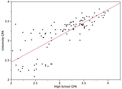
Correlation (2.2)

• What do we examine in a scatterplot to better understand the data?
  • Pattern: form, direction, strength
  • Deviations: outliers
• What types of variables are plotted with a scatterplot?
  • two quantitative variables
• Given the two scatterplots below, which has the stronger relationship?
  • (display two scatterplots of the same data but with different scales)
  • Point out that they are both the same
• What form best fits the scatterplot?
  • (display scatterplot)
  • linear
  • we will now focus on linear relationships to explore some of the numerical measures which can help us further understand the data.
• What numerical measure can we use to measure the strength and direction of a linear relationship between two quantitative variables?
  • correlation coefficient (r)
  • formula: [math]r = \frac{1}{n - 1} \sum_{i=1}^n \left (\frac{(x_i - \bar{x})}{s_x} \right) \left (\frac{(y_i - \bar{x})}{s_y} \right)[/math]
  • discuss some of the ideas in the formula.
  • we will not focus on the formula, but rather on understanding how to interpret r.
• What is the range of possible values for correlation?
  • -1 to 1
  • (draw a horizontal line from -1 to 1.)
• How does the value of r tell us about the direction of the linear relationship?
  • Negative values indicate a negative relationship
  • Positive values indicate a positive relationship
  • (indicate direction info on line)
• How does the value of r tell us about the strength of the linear relationship?
  • Values at or very near zero suggest no relationship between the variables.
  • Values near-ish to 0, but not 0, either positive or negative, indicate a weak relationship.
  • Values near -1 and 1 indicate a strong relationship.
  • (indicate strength info on line)
  • (display image of various scatterplots, with calculated r)
• A correlation requires two quantitative variables, does it matter which is explanatory and response? Why?
  • NO...a correlation measures the relationship between two quantitative variables
• Can we measure a correlation between the chemistry test scores for a group of students and what class they were in? Why?
  • NO...a correlation can only be calculated between two quantitative variables....requires arithmetic in the calculation
• If we change the units of measurement for one of the variables, will the value of r change?
  • No...the pattern of the relationship and the correlation remain the same.
  • In fact the correlation has no units.
  • (display example)
• Does a large correlation indicate that the relationship is linear?
  • NO
  • the scatterplot must be assessed to determine if a linear relationship exists, before using a correlation to describe the data.
  • (display example)
• Which measures of center and spread are used with the correlation? Why?
  • mean and standard deviation
  • correlation is not a resistant measure
• What is the effect of outliers on correlations?
  • r is strongly affected by a few outlying observations
  • use the applet to show how an outlying point affects correlation
• Why doesn’t a tight fit to a horizontal line imply a strong correlation?
  • (draw example.)
  • the value of x is irrelevant to the value of y, the variables are not related.

Scatterplots (2.1)

• What is the most common way to display the relationship between two quantitative variables?
  • a scatterplot
  • display dataset and have student explain how to make one for two quantitative variables...draw on the board
• On which axis should the explanatory variable, if there is one, be plotted? the response variable?
  • expl goes on the x-axis
  • resp goes on the y-axis
• What do we look at when we examine a scatterplot?
  • overall pattern and striking deviations
  • pattern: form, direction, strength
• What types of form might a scatterplot show?
  • (display examples...without labels)
  • linear
  • curvilinear
  • clustered
  • no relationship
• What types of direction might a scatterplot show?
  • (display examples...without labels)
  • positive
  • negative
• How do we determine the strength of a relationship displayed in a scatterplot?
  • (display examples...without labels)
  • by how closely the points follow the form of the relationship
  • how well we can predict y given x
• What deviations might be evident in the data?
  • (display a graph with outliers)
  • outliers
• What does this plot show?
  • (display an example scatterplot)
  • discuss issue of scale (both x and y axis should provide similar variability to points.
• Why might it be useful to add a categorical variable to a scatterplot?
  • (display examples)
  • might show that points are clustered in an important way
  • could even be that relationship is not what it appears
• What sort of graph would we create if we had a categorical explanatory variable and a quantitative response?
  • side by side boxplots
  • draw on board...Actress/Actor Oscar winners explain ages

Examining relationships (Chapt 2 intro)

• What more can we know about the data if we look at two variables together?
  • whether or not the two variables are related, are associated, have a relationship.
  • examples:
    • Are years of education related to personal income?
    • How do SAT scores relate to freshman year grades?
    • Think back to the research questions we came up with on the first day, are any of them proposed two variable relationships?
• If we are measuring two variables, do we collect a different sample of individuals for each variable?
  • NO, the variables must be measured on the same individuals
  • (display dataset) one dataset of observations, with many measurements about each individual
• Two variables may be considered associated if knowing a value of one of the variables.....
  • tells me something about the values of the other variable.
  • Example: a student got an A in Math in one year....what grade would you predict for math in the following year?
• What do we need to know about the dataset and the variables before we can begin examining the relationship?
  • What population and sample are the data obtained from?
  • How are each of the variables measured?
  • Which variables are categorical and which are quantitative.
    • Sometimes categorical measures may be combined to create a quantitative index
    • Other times a quantitative measure may be divided into categories. (e.g., age, proficiency level on a statewide test)
• How might we label the two variables to show the nature of the relationship?
  • response variable - measures an outcome of the study
  • explanatory variable - explains (or causes) changes in the response variable
  • example years of education explains personal income (may or may not cause it)
  • temperature explains hours of sleep (and may even cause it to vary)
• What other terms are used to describe explanatory and response variables?
  • independent and dependent
• We will use the same approach for two variables that we used with one variable. What are the three steps?
  • graphical display
  • examine graph for overall pattern and deviations
  • use numerical summaries to describe specifics of data

Density curves and normal distributions (1.3, through 68-95-99.7 rule)

• What are the first steps of exploratory data analysis, when first presented with a collection of data?
  • plot the data. especially if quantitative (histogram, boxplot)
  • Examine the graph for pattern, and outliers
  • Calculate appropriate summary statistics to describe center and spread
• When we graph a dataset as a histogram, we often see that the shape resembles a smooth mathematical function. What do we call that function.
  • a density curve
  • (display images of variety of density curves)
• What properties of a density curve are noteworthy?
  • it is always on or above the horizontal axis
  • its area under the curve (and above the x-axis) is exactly 1
  • it can be used to approximate an observed histogram created from an actual dataset
  • (display a histogram with curve; demonstrate how area = proportion)
• How can we think about the median of a density curve? the mean?
  • the median is the point with equal area above and below.
  • as the mean is an arithmetic average, we can think of the mean as the point at which the curve would balance
    • easy to see the balance point in a normal curve, more difficult to find the balance point in a skewed curve. (draw one of each)
• As a density curve is idealized, what notation do we use to indicate mean and standard deviation, so we don't get confused with x-bar and sd?
  • μ and σ
• Which density curve will we focus on going forward?
  • the Normal curve
  • the Normal curve describes Normal distributions
  • as for all density curves there is a formula wich we can use to create the curve, but how this works is beyond this class.
• There are many variations of Normal curves. What do they have in common? How do they differ?
  • in-common: symmetric, unimodal, bell-shaped
  • differ: μ and σ (draw a few Normal curves with different μ and σ)
• How do I know how far to draw the distance to represent σ?
  • from the mean to the inflection point on either side of the mean.
• Why are Normal distributions important in statistics?
  • Effective at modeling some distributions of real data (e.g., test scores, repeated measures of the same quantity, characteristics of biological populations), although there are many instances of non-Normal data
  • Good approximations of chance events
  • Statistical inference procedures based on Normal distributions often work well for other roughly symmetric distributions.
• How do we denote a Normal distribution with a particular μ and σ?
  • N(μ, σ)
• What property of the Normal distributions is represented in this graph? How do we use the property?
  • (display example Normal distribution, heights?, with +/- 3 standard deviations delineated)
  • 68-95-99.7 rule
  • 1, 2, and 3 standard deviations encompasses these percentages of data; approximately true for actual data
• In the distribution of heights of young women, what percentage of young women have heights between 62 and 67 inches? What are the height of the middle 95%? What percent of young women have heights greater than 72 inches?
  • btwn 62 and 67: 68%
  • middle 95%: 59.5-69.5
  • above 72: 2.5%

Displaying distributions with numbers (1.2)

• What aspects of a histogram do we examine to better understand our quantitative data?
  • overall pattern: shape, center, spread
  • deviations: outliers
• In this section, we will examine numerical descriptions which may help us better understand our data. What statistics do we use to measure the center?
  • mean, median
• How do these two values differ?
  • mean is average value
  • median is middle value
• How do we calculate the mean?
  • [math]\bar{x} = \frac{x_1 + x_2 + ... * x_n}{n} = \frac{1}{n} \sum{x_i}[/math]
  • carefully review the notations (x-bar, summation, subscripts...no order implied), emphasizing that this is an average
  • (display best actress Oscar winner calculation)
• How do we calculate the median?
  • Find the midpoint of the distribution, such that half of the observations are below and half are above
  • If the number of observations is odd, the median is the observation at the center of the ordered list of observations
  • If the number of observations is even, the median is the half-way point between the two center observations in the ordered list.
  • (Display the best actress Oscar winner calculation)
• What is the median of 9, 4, 2, 3, 5, 8, 1?
  • 4
  • order the numbers into an ordered list to show the concept
• What is the median of 9, 4, 2, 3, 5, 8, 1, 8?
  • 4.5
  • add the additional 8 into the ordered list.
• How will an outlier in the data effect the mean and median?
  • (Display two simple datasets, with the second having an obvious outlier/data entry error. Provide mean/median for each x-bar_A=68.14, x-bar_B=162)
  • It will result in a mean which is closer to the outlier, than if the outlier is not there.
  • It will not change the median, accept that it is a data point in the upper or lower half.
• How will the mean and median compare for a skewed distribution?
  • (Display images of distributions with mean and median indicated.)
  • The mean will be farther along the tail of the distribution, while the median is closer to the bulk of the data.
• What can we conclude about the mean, as a measurement tool?
  • It is not a resistant measure, as it is strongly influenced by extreme values
• With what kinds of data should we use the mean as a measure of center?
  • Symmetric distributions with no outliers
• In our examination of the overall pattern in our data, we have discussed shape and center. What's left?
  • spread or variability
  • (display image of two distributions with different variability, but the same center)
• What are some ways we might quantify spread
  • range (max-min), inter-quartile range (IQR, distance between 25th and 75th percentiles), standard deviation
• What is the range?
  • Exact difference between largest and smallest observations
  • [math]Range = Max - Min[/math]
  • (display best actress Oscar winner calculation)
• If the median breaks the data into halves, how do the quartiles divide the data
  • into quarters or fourths.
• How do we find the quartiles for a dataset?
  • After locating the median, find the center observation in the lower and upper halves.
  • The lower half is Q1
  • The upper half is Q2
  • (draw a line representing range of data, from min to max; label M, Q1, Q2, 25% in each section, middle 50%, IQR)
  • (display IQR calculations for best actress Oscar winners dataset)
  • There are a number of other ways to calculate percentiles; different software apps do it differently.
• What is Q1 and Q3 in terms of percentiles?
  • 25th and 75th
• What do we mean by percentile?
  • The percent of observations which occur at or below that value.
• How can we use the IQR to help us identify outliers?
  • Calculate Q1 - (1.5 * IQR), Q3 + (1.5 * IQR); any values which lie outside these upper and lower thresholds may be considered outliers.
  • (display histogram for best actress Oscar winners, with potential outliers noted)
  • calculate outlier thresholds
    • Q1=32 and Q3=41.5 ⇒ IQR=9.5
    • Q1 − 1.5(IQR) = 32 − (1.5)(9.5) = 17.75
    • Q3 + 1.5(IQR) = 41.5 + (1.5)(9.5) = 55.75
    • The three largest values in the dataset may be considered outliers.
• What are the three options for how to handle an outlier?
  • Keep it....the observation belongs to the population we are studying...example: outliers in best actress Oscar winners
  • Drop it....the observation is fundamentally different from the other observations; didn't realize when data was collected...example: studying typical third graders, but dataset includes observation for student who is two grades ahead. Student could well be an outlier on many physical characteritics (low), as well as cognitive measures (high), and likely does not represent typical third graders
  • Fix it...check the original data collection process to see if the observation is a data error.
• What 5 numbers, of those which we have talked about so far, would fit nicely together to make a 5-number summary?
  • Min, Q1, M, Q3, Max
  • the five number summary for best actress Oscar winners is: 21, 32, 35, 41.5, 80. (compare to histogram)
• What graph can we use to visually display the five-number summary?
  • a boxplot
  • construct a box plot using the best actress data, y axis Age 20-80:
    • 5-number summary 21, 32, 35, 41.5, 80
    • outliers: 61, 74, 80
    • largest observation that is not an outlier 49
• How might we organize our boxplots if we had both actress and actor data?
  • side-by-side
  • (display side-by-side boxplot for oscar winners; interpret what the graph says about the data)
• We've discussed range and IQR, which are both useful when our measure of center is a median. What measure of spread is useful when the measure of center is the mean?
  • standard deviation
• How does the standard deviation show the spread of the data?
  • It quantifies how far the observations are from the mean.
  • many notations: SD, s, Sd, StDev
• If we have a small set of data, no. of people who enter a pet store in 8 consecutive hours: 7, 9, 5, 13, 3, 11, 15, 9, and we've calculated the mean: 9, what's the first step in calculating an SD?
  • write out the data on a line, show the mean
  • subtract each observation from the mean
• What do we do next?
  • square each deviation
  • if we sum the deviations, we get 0; we could use the absolute deviation...
• Once we have the squared deviations, what could we do to summarize them...to find the average squared deviation?
  • sum them up, and divide by the number of observations
  • but in fact we divide by n-1, because that's how many unique pieces of information we have. It's called degrees of freedom...
  • sum of squared deviations = 112, divided by 7 is 16
• Now we have the average squared deviation. What could we do to help us better understand the number?
  • Take the square root, as now the number is on the same scale as the original data....same units
  • [math]sd = \sqrt{16} = 4[/math]
  • The formula is [math]sd = \sqrt{\frac{1}{n-1}\sum (x_i - \bar{x}_i)^2}[/math]
• When should we use sd?
  • it goes with the mean, best used with symmetric distributions with no outliers
• When is sd = 0?
  • when all of the observations are the same value...there is no spread
• Is sd a resistant measure?
  • no, large deviations from the mean will result in a large sd, larger than the other values would suggest
• What is the single best way to describe a dataset?
  • a graph, numerical summaries don't provide as much depth of information (as they summarize the data)
• Is it OK to make a linear change to a measurement scale for a variable?
  • yes, always.
  • you can easily apply a linear trasnformation in SPSS and in spreadsheets, e.g., if you need to change the unit of measurement
• Will the shape, center and spread of the distribution remain the same for a transformed variable?
  • shape: it will have the same basic shape: skewed, symmetric, unimodal, etc.
  • center and spread: no, but they will change in a systematic way

Displaying distributions with graphs (1.1)

• Let's examine the data from a survey which asked 1200 US college students about how they perceive their body: overweight, underweight, or about right. Here is what the data would look like in a spreadsheet. (display printscreen of body image spreadsheet) What would be a good starting point for organizing our data?
  • count how many individuals are in each group
  • note that with 1200 individuals in the dataset, there's too much data to make any sense of it in the spreadsheet format.
  • be sure to review the set up of the spreadsheet: how many variables, which is the variable we are focused on?
• What do we call a data display which shows the values and counts (or percents) for a variable?
  • frequency distribution or frequency table
  • display freq dist for body image data...note that percents don't add to 100%
• What graph(s) could we use to visualize the data?
  • bar graph and pie chart
  • display body image graphs
• What if we collected data as to what kind of pet a person has and the options are: dog, cat, fish, reptile. Does it make sense to graph this data on a bar graph? on a pie chart?
  • Yes for a bar graph, because you don't need to account for all of the options, you could display the number of people who have each kind of pet
  • No for a pie chart, because the categories don't cover everyone. Some people will have other kinds of pets (e.g., pigs) and some will have no pets. The categories in a pie chart must be all of the options which make up the whole amount.
• Could you transform a table of the percent of children living in poverty for 35 economically advanced countries into a bar graph? into a pie chart? why?
  • yes for a bar chart, because it's reasonable to compare the percents across countries. (see example on next slide)
    • note that countries are organized by increasing percent....would the graph be as useful if the countries were listed alphabetically?
  • no for a pie chart, not because we don't have everything...we have all 35 countries, but because the percents are within each country...for children living in Finland, what percent are living in poverty? These are conditional percents, which we will discuss in chapter 2.
• When we have quantitative (numerical) data, what can we do to help us better understand the data?
  • assuming we already understand the context of the data, graph it and look for general patterns and anomalies.
• What kinds of graphs are useful when we want to visualize quantitative data?
  • histograms and stemplots
    • use these for visualizing one variable at a time, to look at the pattern of spread in the data
  • time plots (a type of line graph)
    • use these when the data are sequenced, e.g., in time
• What kind of graph is the standard for use in visualizing the data for one quantitative variable?
  • The histogram
  • It breaks the range of data into classes (intervals) and displays the count or percent of observations in each class.
  • (display example of histogram from ips6e)
  • discuss axes, classes/bins/intervals, area of bars represents how much data is present in class, bars together, shape, anomalies
• How many classes (also called bins) should be included in a histogram? (include link to applet)
  • No standard.
  • show how changes in class width change our interpretation of the data
  • Software will use defaults, which you can change--as you get more practiced at creating these, you will have a better sense of what will help you best visualize the data.
• What kind of graph is useful when you have a quantitative variable, which has positive values, and a small number of observations?
  • stemplot (stem and leaf plot)
• Let's make a stemplot
  • Collect the age of the youngest person living in the household of each student
  • Create stems
  • put on leaves
  • Display back to back stemplot; useful, but we will study boxplots next week which are more useful still
• Which is more useful, generally speaking, histogram or stemplot?
  • histogram
  • stemplot is useful when your only tool is pencil and paper; not used in research journals
• What is the purpose of making a statistical graph?
  • to better understand the data
• What do we look for when we examine a graph?
  • overall pattern: shape, center, spread
  • deviations from pattern: outliers
  • Put up a few examples to discuss the following terms:
    • modes, unimodal, bimodal
    • symmetric....unimodal, bimodal, uniform
    • tails
    • skewness: skewed right (salary), skewed left (age at death-natural causes)
    • center: midpoint
    • spread: variability (min, max)
    • outliers
• Why should we pay particular attention to outliers?
  • because that particular observation may be systematically different from the others: data entry error, equipment failure, different unit of measure, an individual which could be considered different than all of the others....does not belong in the same population.
  • display graph showing outlier
• Why would we want to make a time plot for a quantitative variable?
  • When the data collected is sequenced in some way, including the sequencing variable in the graph often changes our interpretation of the data.
  • Show example timeplot, time is on the horizontal axis, lines connect the data points, may also include a trend line.

Chapt 1.Introduction

• What is/are statistics? (ask a number of students for their ideas)
  • wp: the study of the collection, organization, analysis, interpretation, and presentation of data...often large amounts of data.
  • numbers derived from data which help us better understand the data....which provide us useful information
• What is data?
  • numerical facts about individuals, cases, or subjects
  • but just looking at all the individual numbers won't help us understand
  • we need to examine the data within the context of a research question
• Example research questions
  • Have students pair up and devise a research question, on any topic
  • Each group presents their question (write it on the board, using the term population where possible)
  • Go back through the questions and identify what numerical facts could be obtained to create the data.
• The big picture of statistics.
  • present the 4 stages described in OLI statistics
  • We want to study a population, but too big
  • Choose a sample and collect data (called producing data)
  • Once we have the data, we need to begin to make sense of or summarize the data (exploratory data analysis)
  • In order to make a conclusion about the population we have to explore how the sample compares to it (using probability)
  • Finally we can use our sample to make a conclusion about the population (inference)
  • We will explore steps 1-3 in Stat Methods I; step 4, inference, is tackled in Stat Methods II
  • We will begin our study of statistics with exploratory data analysis (EDA), chapters 1 and 2 in the text.
• Looking back at our research questions, I see that we want to obtain data about a number characteristics for each individual in our population or sample. What math term do we use to name these characteristics?
  • variables
  • a variable is any characteristic of an individual
• What do we call a particular collection of numerical facts about individuals?
  • a dataset, identified with particular circumstances
• A dataset may be displayed as a grid of rows and columns. In the example where are the individuals? Where are the variables?
  • Display an example
• As we established, a data set is identified with particular circumstances. What are some questions we should know about this example dataset?
  • What questions are we looking to answer with this data?
  • What population are we interested in?
  • Who are the individuals in the dataset?
  • How many are there?
  • How many variables do the data contain?
  • What is the definition of each of the variables?
  • How were the values in these variables obtained?
• How are the variables for gender (M, F) and test score (0-100 pts) different?
  • gender classifies each individual into a category-->Categorical variable
  • test score provides a numerical value or measurement for each individual-->Quantitative variable
• Label the variables in the dataset below as either categorical or quantitative
  • display example dataset
• What problem do we have if we only know the the names and values of the variables in a dataset?
  • Display new example and discuss what each of the variables might mean.
  • Discuss issues with measurement and assigning categories.
    • reliability/validity of measurement instrument
    • assigning meaningful categories
    • categories which are coded using numbers
    • counts vs. rate of occurrence
• Let's get started with exploratory data analysis; two types
  • distributions of individual variables
  • relationships between two variables
• In each case we will look at
  • visual displays of data (graphs/charts)
  • numerical summaries/measures