Types or Concepts of Equilibrium
MICROECONOMICS

|
Concept of Equilibrium |
| The word equilibrium is derived from the Latin word aequilibrium which means equal balance. Its use in economics is imported from physics. In physics it means a state of even balance in which opposing forces or tendencies neutralize each other. Prof. Stigler defines equilibrium in his sense in these words:" equilibrium is a position from which there is no net tendency to move, we say net tendency to emphasize the fact that it is not necessarily a state at sudden inertia but may instead represent the cancellation of power forces. In economics, equilibrium implies a position of rest characterized by absence of change.
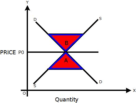
Market equilibrium, for example, refers to a condition where a market price is established through competition such that the amount of goods or services sought by buyers is equal to the amount of goods or services produced by sellers. It is the point at which quantity demanded and quantities supplied are equal. This price is often called the equilibrium price or market[1]clearing price and will tend not to change unless demand or supply change. |
Price of market balance:
- P - price
- Q - quantity of good
- S - supply
- D - demand
- P0 - price of market balance
- A - surplus of demand - when P<P0
- B - surplus of supply - when P>P0
| Static Equilibrium |
"According to Prof. Mehta". "Static equilibrium is that equilibrium which maintains itself outside the period of time under consideration ". It is state of bliss which every individual firm, industry or factor wants to attain and once reached, would not like to leave. Consumer is in equilibrium when he gets maximum satisfaction from a given expenditure on different goods and services.Any move on this part to reallocate his expenditure among his purchases will decrease rather than increase his total satisfaction. A firm is in equilibrium when its profit is the maximum and it has no incentive to expand or contract its output. It is a position in which neither the adjusting firms have any tendency to live nor for new firms to enter the industry. In other words, an industry is in equilibrium when all firms are earning only normal profits.
Static equilibrium is of three types:
- Micro static.
- Macro static and
- Comparative static
| Micro static: |
An economic model refers to relationship among different variables in which one variable appears in more than one relationship. In the micro static models of price determination, supply and demand relationship determine price at a point of time which are also constant through time. The given demand and supply functions are
Where,
D = demand
P = price
S = supply
The equation I shows that demand is inversely proportional to price i.e. if price decrease the demand will rise and if price increases, the demand will fall keeping other things constant. On the other hand equation II shows that supply is also the function of price i.e. if price increase supply will rise and if price decrease supply will fall, other things remaining constant.
The micro static relationship is illustrated with the help of diagram.
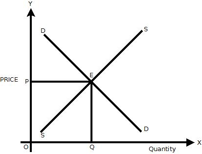
The above diagram shows DD and SS the demand and supply curves respectively. They intersect at point E where quantities of demand and supplied equals to OQ at price OP. This is static analysis of price determination, for all variables such as quantity supplied, quantity demanded and price refer to the same point or period of time.
Generally, the economists are interested in the equilibrium values of the variables which are attained as a result of the adjustment of the given variables to each other. That is why economic theory has sometimes been called equilibrium analysis. Till recently, the whole price theory in which we explain the determination of equilibrium prices of the products and factors in different market categories were mainly static analysis. The values of the various variables such as demand, supply, and price were taken to be relating to the same point or period of time.
| Macro-Static: |
The concept of Macro-Static explains the static equilibrium position of the economy. This concept is best explained by Prof. Kurihara in these words: “If the object is to show a still picture of the economy as a whole, the macro-static method is the appropriate technique.. This technique is one of investigating the relations between macro-variables in final position of equilibrium without reference to the process of adjustment implicit in that final position”. Such a final position of equilibrium may be shown by the equation Y = C + I
Where, Y = Total Income
C = Total consumption expenditure
I = Total Investment expenditure
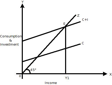
In a static Keynesian model, the level of equilibrium is determined by the interaction of aggregate supply function and the aggregate demand function. In diagram OZ shows aggregate supply function and C + I line represents aggregate demand function. The line OZ and C + I intersect at point E, which determines equilibrium level of income at OY1. It simply shows a timeless identity equation without any adjusting mechanism.
| Comparative Static: |
A Comparative Static analysis compares one equilibrium position with another when data have changed and system has finally reached another equilibrium position. It does not show how the system has reached the final equilibrium position with a change in data. It merely explains and compares the initial equilibrium position with the final one reached after the system has adjusted to a change in data.
Thus, in comparative static analysis, equilibrium positions corresponding to different sets of data are compared.
Let us see few examples of comparative static analyses.
Consider our previous example of static analysis of demand and supply which determine the equilibrium quantity and price. We can thus think of an analysis in which we start with a system in equilibrium. We now introduce a change and study the ultimate effect of a change. This can be explained with the following diagram
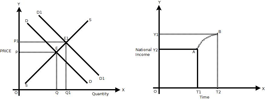
The original equilibrium between DD the demand curve and SS the supply curve is at E1. When demand increases to D1D1, as a result of increase in income, the new equilibrium is at E2 at the price OP2. In comparative static analysis, we are concerned only with explaining the new equilibrium position at point E2 and comparing it with E1. We are not concerned with the whole path the system has travelled from E1 to E2. Alfred Marshall has made extensive use of comparative static in his time-period analysis of pricing under perfect competition.
Although the dynamic analysis of the two equilibrium positions with different sets of data is more comprehensive and informative.
Limitations of Comparative Statics Analysis
- It fails to predict the path which the market follows when moving from one equilibrium position to another.
- It cannot predict whether or not a given equilibrium position will ever be achieved. For this purpose we need dynamic analysis.
| Dynamic Equilibrium |
When after a fixed period the equilibrium state is disturbed it is called dynamic equilibrium.
In dynamic equilibrium prices, quantities, incomes, tastes, technology etc are constantly changing.
For e.g. suppose some more persons develop the taste for fish, s a result the demand for fish will increase seller will at once raise the price and thus change the behavior of the old buyers. The market will be thrown into a state of disequilibrium and will remain so till the supply of fish is increased to the level of the new demand. When new equilibrium will be brought in by the forces contenting forces.
The word dynamic means causing to move. In economics, ‘dynamic’ refers to the study of economic change. The essence of any knowledge lies in formulating relationships between phenomena. There must be thus sequence of events for the knowledge to be born. The main purpose is to know as to how complex of current events will shape itself I the future. To do so it is necessary to visualize the way it has itself arisen out of the past events. The moment we talk of sequence of events, the elements of time creeps into our analysis. Economics is thus a process of change through time.
Dynamic equilibrium is of two types
- Micro Dynamic equilibrium
- Macro Dynamic equilibrium
| Micro-Dynamics (cobweb) |
It is used to explain the dynamics of demand, supply and price over long period of time. The cob-web model (or Theorem) analyses the movements of prices and outputs when supply is wholly determined by prices in the previous period.
As prices moves up and down in cycles, quantities produced and also seem to move up and down in a counter-cyclical manner (e.g. prices of perishable commodities like vegetables).
In order to find out the conditions for converging, diverging or constant cycles: one has to look at the slope of the demand curve and then of the supply curve.
Assumption
- The cob-web Model is based on the following assumption:
- The current year’s (t) supply depends on the last year’s (t-1) decisions regarding output level.
- Hence current output is influenced by last year’s price. i.e. P (t-1)
- The current period or year is divided into sub-periods of a week or fortnight.
- The parameters determining the supply function have constant values over a series of periods.
- Current demand (Dt) for the commodity is a function of current price (Pt).
- The price expected to rule I the current period is the actual price in the last year.
- The commodity under consideration is perishable and can be stored only for one year.
- Both supply and demand function are linear .i.e. both are straight line curves which increases or decreases at a constant proportion.
The Cob-web Model
There are two types of Cob-web Models:
- Convergent
- Divergent
- Continuous
(1) Convergent Cob-web
Under this model the supply is a function of previous year i.e. S= f (t-1) (‘t’ is the current period and‘t-1’ is a previous period) and on the other hand the demand is the function of price i.e. Dt=f (P). The equality between the quantity supplied and quantity demand is called as Market equilibrium.i.e. St=Dt. Equilibrium can be established only through a series of adjustment if current supply is in response to the price during the last year. But this adjustment will take place over a several consecutive periods.
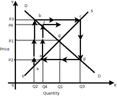
For e.g. suppose we take the example of onion growers who is producing one crop in a year. The onion growers will grow this year on the assumption that the price of onions this year will be equal to price in the last year. The market demand and supply curves for onions are represented by DD and SS curves respectively in diagram.
Suppose the price in the last year was OP1 and Producers decide the equilibrium output OQ1 this year. Now suppose there is crop failure due to natural calamities which decrease the output OQ2 which is less than OQ1 (i.e. equilibrium output). Lack of supply will increase the price to OP2 in the current period. In the next period, the onion growers will produce OQ3 quantity in response to the higher price OP2.But this is more than the equilibrium quantity OQ1 which is the actual need of the market. The excess supply will lower the price to OP3. This will encourage the producer to change the producer plan, where they will reduce the supply to OQ4 in the third period. But this quantity is less than the equilibrium quantity OQ1. This will lead to again rise in price to OP4, which in turn will encourage the producers to produceOQ1 quantity. The equilibrium will be established at point g where DD and SS curves intersect. This series of adjustments from point a,b,c,d,and e to f is traced out as a cobweb pattern which converge towards the point of market equilibrium g. This is also called as the dynamic equilibrium with lagged adjustment.
(2) Divergent Cob-Web
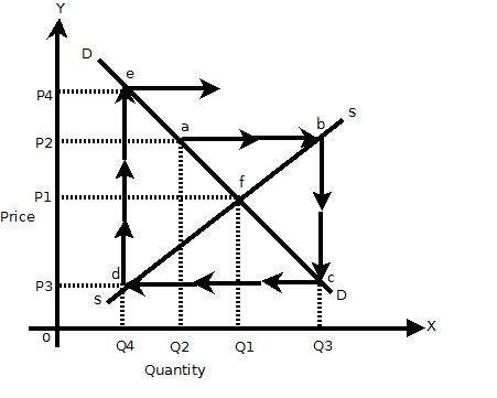
The divergent cob-web is unstable cobweb when price and quantity changes move away from the equilibrium posting. This can be explained with the help of following diagram,
We will start with the initial equilibrium price is OP1 and equilibrium quantity OQ1. Now suppose there is a temporary disturbance that causes output to fall to OQ2. Due to lack of supply the price will rise to OP2.
The increase in price will in turn raise the output to OQ3 which is more than the equilibrium output OQ1. The increase in supply will lead to fall in price to OP3. This fall in price will increase the demand and there will be excess demandOQ2 than supply. The excess demand will shoot up the price to OP4. This shows that the price will be still away from the equilibrium after the adjustment by the producers. This is called as Divergent cob-web.
(3) Continuous cob-web
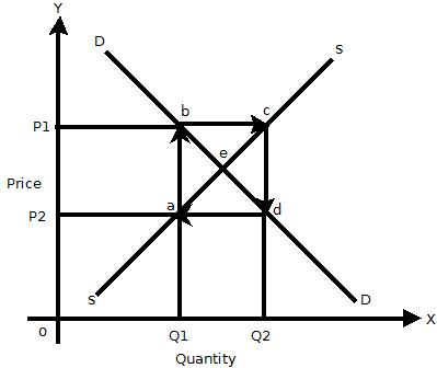
The cob-web models in this show the continuous changes in price and quantities.
Suppose we start with the price OP1 as shown in the diagram. As the supply will be more due to high price in the market. On the other hand the demand will be less as compared to the supply OQ2 and the demand will reduced to OQ2. The fall in demand will force the producer to decrease price to OP2 in next period. But at this price OP2 the demand will be OQ2 which is more than the supply OQ1 which reduced. This way the prices and quantities will circulate constantly around the equilibrium.| Macro-Dynamics (cobweb) |
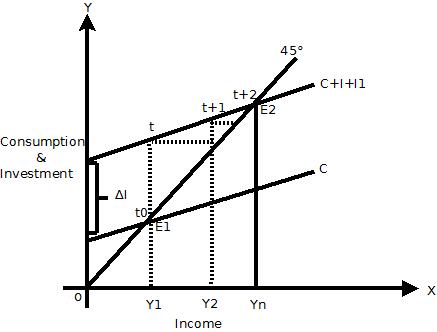
According to Kurihara,” ‘Macro-Dynamics’ treats discrete movements or rates of change of macro-variables. It can be explained in terms of the Keynesian process of income propagation (the investment multiplier) where consumption depends on income i.e. C = f (Yt-1)
Where
C = Consumption
Y = Income
f = function
The function shows that the consumption in the current period (t) depends on the Y in the previous period (t-1). On the other hand investment is a function of time and of constant autonomous investment ∆I (Autonomous investment is the investment which does not changes due to changes in income.i.e. changes in investment does not take place due to change in income).For e.g. government does the investment for welfare of the people and not for profit expectation. So investment function can be written as It = f (∆ I). This can be explained with the following diagram.
The above diagram shows that C is the aggregate demand function and 450 degree line is the aggregate supply function. Suppose we start with the time period t0 where with an equilibrium level of income OY1, investment increased from I0 to I1, this can be seen by the new aggregate demand function line C + I + I1.But in period t, consumption lags behind and it is still on the equilibrium point E1. In next period t + 1 consumption increased with the increase in investment, which lead to increase in income from OY1 to OY2. This is the process of income prorogation which will continue till the aggregate demand function C + I + I1 intersects the aggregate function 450 line at point E2 in the nth period. The new equilibrium level of income is at OYn. The curved steps from t0 to E2 show the macro-dynamic equilibrium path.
(1) Stable Equilibrium
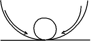
Equilibrium is said to be stable when the economy is disturbed on which it depends and again resume to its original position that is the disturbance in the equilibrium is self adjusting so that the original equilibrium is restored. This stable equilibrium can be seen with the diagram. In words of Marshall “When the demand price is equal to the supply price, the amount produced has no tendency either to be increased or to be diminished, it is an equilibrium. Such equilibrium is stable: that is, the price, if displaced a little from it, will tend to return, as a pendulum oscillates about its lowest point. Another famous simile is that of a bowl and a bowl given by Schumpeter. A bowl that rest in a bowl is in stable equilibrium because if disturbed it will eventually come to the rest in its initial position after moving back and forth.
(2) Unstable Equilibrium
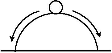
In case of unstable equilibrium the disturbance in the economy will lead or exaggerate the further disturbances will never to its original position.In Pigou’s words, “If the small disturbance calls out further disturbing forces which act in a cumulative manner to drive the system from its initial postion,” it is in unstable equilibrium. “As an egg if balanced on one of its ends would at the smallest shake fall down, and lie length ways, “as pointed out by Marshall. If the bowl is inverted and the ball is perched on its top, it will be in unstable equilibrium. For once the ball is pushed; it falls off the top of the bowl to the ground and does not return to its original position, as shown in figure.
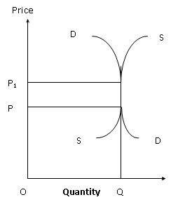
Another type of equilibrium generally referred to is neutral equilibrium.According to Prof. Pigou, “An egg lying on its side is in neutral equilibrium.” The static neutral equilibrium condition is illustrated in fig. and the dynamic in figure. In fig E is the initial equilibrium point where OQ quantity is demanded and supplied at OP price. With the rise in the price to OP1, E1 becomes the new equilibrium point but the quantity demanded and supplied remains the same, i.e. OQ. Thus, the price range PP1 (=EE1) represents neutral equilibrium.Neutral equilibrium is when the disturbing forces neither bring it back to the original position nor do they drive it further away from it. It rests where it has been moved. Thus, in the case of a neutral equilibrium, the object assumes once for all a new position after the original position is disturbed.
(3) Neutral Equilibrium
Neutral equilibrium is when the disturbing forces neither bring it back to the original position nor do they drive it further away from it. It rests where it has been moved. When an initial equilibrium position is disturbed, the forces of disturbance bring it to the new position of equilibrium where the system has come to rest. A ball on the billiard table if disturbed will come to rest at the new position to which it has moved. According to Prof. Pigou, “An egg lying on its side is in neutral equilibrium.” The static neutral equilibrium condition is illustrated in figure.
In fig E is the initial equilibrium point where OQ quantity is demanded and supplied at OP price. With the rise in the price to OP1, E1 becomes the new equilibrium point but the quantity demanded and supplied remains the same, i.e. OQ. Thus, the price range PP1 (=EE1) represents neutral equilibrium.
| Partial Equilibrium |
Partial equilibrium analysis is the analysis of an equilibrium position for a sector of the economy or for one or several partial groups of the economic unit corresponding to a particular set of data.Partial or particular equilibrium analysis, also known as micro economic analysis, is the study of the equilibrium position of an individual, a firm, an industry or a group of industries viewed in isolation. In other words, this method considers the changes in one or two variables keeping all others constant, i.e., ceteris paribus (others remaining the same). The ceteris paribus is the crux of partial equilibrium analysis.For Example
(a) Consumer’s Equilibrium: With the application of partial equilibrium analysis, consumer’s equilibrium is indicated when he is getting maximum aggregate satisfaction from a given expenditure and in a given set of conditions relating to price and supply of the commodity.
The conditions are: 1) the marginal utility of each good is equal to its price (P), i.e.
And (2) the consumer must spend his entire income (Y) on the purchase of goods, i.e.
It is assumed that his tastes, preferences, money income and the prices of the goods he wants to buy are given and constant.
(b) Producer's Equilibrium: A producer is in equilibrium when he is able to maximise his aggregate net profit in the economic conditions in which he is working.
(c) Firm's Equilibrium: A firm is said to be in long-run equilibrium when it has attained the optimum size when is ideal from the viewpoint of profit and utilization of resources at its disposal.
(c) Industry's Equilibrium: Equilibrium of an industry shows that there is no incentive for new firms to enter it or for the existing firms to leave it. This will happen when the marginal firm in the industry is making only normal profit, neither more nor less. In all these cases; those who have incentive to change it have no opportunity and those who have the opportunity have no incentive.
*Assumptions
- Commodity price is given and constant for the consumers.
- Consumer’s taste and preferences, habits, incomes are also considered to be constant.
- Prices of prolific resources of a commodity and that of other related goods (substitute or complimentary) are known as well as constant.
- Industry is easily availed with factors of production at a known and constant price compliant with the methods of production in use.
- Prices of the products that the factor of production helps in producing and the price and quantity of other factors are known and constant.
- There is perfect mobility of factors of production between occupation and places.
| General Equilibrium |
Leon Walras (1834-1910), a Neoclassical economist, in his book ‘Elements of Pure Economics’, created his theoretical and mathematical model of General Equilibrium as a means of integrating both the effects of demand and supply side forces in the whole economy.Elements of Pure Economics provides a succession of models, each taking into account more aspects of a real economy.General equilibrium theory is a branch of theoretical microeconomics.The partial equilibrium analysis studies the relationship between only selected few variables, keeping others unchanged.Whereas the general equilibrium analysis enables us to study the behaviour of economic variables taking full account of the interaction between those variables and the rest of the economy.In partial equilibrium analysis, the determination of the price of a good is simplified by just looking at the price of one good, and assuming that the prices of all other goods remain constant. Thus the economy is in general equilibrium when commodity prices make each demand equal to its supply and factor prices make the demand for each factor equal to its supply so that all product markets and factor markets are simultaneously in equilibrium.Such a general equilibrium is characterized by two conditions in which the set of prices in all product and factor markets is such that
1) All consumers maximize their satisfactions and all producers maximize their profits and
2) All markets are cleared which means that the total amount demanded equals the total amount supplied at a positive price in both the product and factor markets.
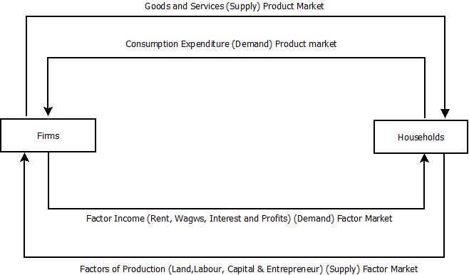
To explain it, we begin with a simple hypothetical economy where there are only two sectors, the household and the business. The economic activity takes the form of flow of goods and services between these two sectors and monetary flow between them. These two flows, called real and monetary are shown in figure.
Where the product market is show in the upper portion and the factor market in the lower portion. In the product market, consumers (Household) purchase goods and services from producers (Firms) while in the factor market, consumers receive income from the former for providing Factor services. The producers, in turn, make payments to consumers for the services rendered i.e. wage payments for labour services, interest for capital supplied, etc. thus payments go around in a circular manner from producers to consumers and from consumers to produces, as shown by arrows in the inner portion of the figure. There are also flows of goods and services in the opposite direction to the money payments flows. Goods flow from the business sector to the household sector in the product market, and services flow from the household sector to the business sector in the factor market, as shown in the outer portion of the figure. These two flows are linked by product prices and factor prices. The economy is in general equilibrium when a set of prices is allowed at which the magnitude of income flow from producers to consumers is equal to the magnitude of the money expenditure from consumers to producers.

|
Activity |
| TRY OUT THIS QUIZ | |
[Activity]

|
Key Terms |
Economic equilibrium.
Stable equilibrium.
Unstable equilibrium.
partial equilibrium.
General equilibrium

|
References and Bibliography |
Ahuja, H.L, ‘Modern Microeconomics- Theory and Applications’
Arrow, K. J. and G. Debreu, ‘Existence of an Equilibrium for a competitive economy’
Arrow, K. J. and F. H. Hahn, ‘General Competitive Analysis’
Koutsoyiannis, A, ‘Modern Microeconomics’
Walras Leon, ‘Elements of Pure Economics’, trans. Jaffe
Johnson, H. G., ‘Two Sector Model of General Equilibrium’
Marshall, Alfred, ‘Principles of Economics’
Simpson, D., ‘General Equilibrium Analysis’
Weintraub, E. Roy, ‘General Equilibrium Theory’


